Binomial heap

Last updated

Binomial heap
Type heap
Invented1978
Invented byJean Vuillemin
Complexities in big O notation
Space complexity
Time complexity
Function Amortized Worst Case
InsertΘ(1) O(log n)
Find-minΘ(1) O(1)
Delete-minΘ(log n) O(log n)
Decrease-keyΘ(log n) O(log n)
MergeΘ(log n) O(log n)

In computer science, a binomial heap is a data structure that acts as a priority queue. It is an example of a mergeable heap (also called meldable heap), as it supports merging two heaps in logarithmic time. It is implemented as a heap similar to a binary heap but using a special tree structure that is different from the complete binary trees used by binary heaps. [1] Binomial heaps were invented in 1978 by Jean Vuillemin. [1] [2]

Contents

Binomial heap

A binomial heap is implemented as a set of binomial trees (compare with a binary heap, which has a shape of a single binary tree), which are defined recursively as follows: [1]

Binomial trees of order 0 to 3: Each tree has a root node with subtrees of all lower ordered binomial trees, which have been highlighted. For example, the order 3 binomial tree is connected to an order 2, 1, and 0 (highlighted as blue, green and red respectively) binomial tree. Binomial Trees.svg
Binomial trees of order 0 to 3: Each tree has a root node with subtrees of all lower ordered binomial trees, which have been highlighted. For example, the order 3 binomial tree is connected to an order 2, 1, and 0 (highlighted as blue, green and red respectively) binomial tree.

A binomial tree of order has nodes, and height . The name comes from the shape: a binomial tree of order has nodes at depth , a binomial coefficient. Because of its structure, a binomial tree of order can be constructed from two trees of order by attaching one of them as the leftmost child of the root of the other tree. This feature is central to the merge operation of a binomial heap, which is its major advantage over other conventional heaps. [1] [3]

Structure of a binomial heap

A binomial heap is implemented as a set of binomial trees that satisfy the binomial heap properties: [1]

The first property ensures that the root of each binomial tree contains the smallest key in the tree. It follows that the smallest key in the entire heap is one of the roots. [1]

The second property implies that a binomial heap with nodes consists of at most binomial trees, where is the binary logarithm. The number and orders of these trees are uniquely determined by the number of nodes : there is one binomial tree for each nonzero bit in the binary representation of the number . For example, the decimal number 13 is 1101 in binary, , and thus a binomial heap with 13 nodes will consist of three binomial trees of orders 3, 2, and 0 (see figure below). [1] [3]

Example of a binomial heap containing 13 nodes with distinct keys. The heap consists of three binomial trees with orders 0, 2, and 3. Binomial-heap-13.svg
Example of a binomial heap containing 13 nodes with distinct keys. The heap consists of three binomial trees with orders 0, 2, and 3.

The number of different ways that items with distinct keys can be arranged into a binomial heap equals the largest odd divisor of . For these numbers are

1, 1, 3, 3, 15, 45, 315, 315, 2835, 14175, ... (sequence A049606 in the OEIS )

If the items are inserted into a binomial heap in a uniformly random order, each of these arrangements is equally likely. [3]

Implementation

Because no operation requires random access to the root nodes of the binomial trees, the roots of the binomial trees can be stored in a linked list, ordered by increasing order of the tree. Because the number of children for each node is variable, it does not work well for each node to have separate links to each of its children, as would be common in a binary tree; instead, it is possible to implement this tree using links from each node to its highest-order child in the tree, and to its sibling of the next smaller order than it. These sibling pointers can be interpreted as the next pointers in a linked list of the children of each node, but with the opposite order from the linked list of roots: from largest to smallest order, rather than vice versa. This representation allows two trees of the same order to be linked together, making a tree of the next larger order, in constant time. [1] [3]

Merge

To merge two binomial trees of the same order, first compare the root key. Since 7>3, the black tree on the left (with root node 7) is attached to the grey tree on the right (with root node 3) as a subtree. The result is a tree of order 3. Binomial heap merge1.svg
To merge two binomial trees of the same order, first compare the root key. Since 7>3, the black tree on the left (with root node 7) is attached to the grey tree on the right (with root node 3) as a subtree. The result is a tree of order 3.

The operation of merging two heaps is used as a subroutine in most other operations. A basic subroutine within this procedure merges pairs of binomial trees of the same order. This may be done by comparing the keys at the roots of the two trees (the smallest keys in both trees). The root node with the larger key is made into a child of the root node with the smaller key, increasing its order by one: [1] [3]

function mergeTree(p, q)     if p.root.key <= q.root.key         return p.addSubTree(q)     elsereturn q.addSubTree(p)
This shows the merger of two binomial heaps. This is accomplished by merging two binomial trees of the same order one by one. If the resulting merged tree has the same order as one binomial tree in one of the two heaps, then those two are merged again. Binomial heap merge2.svg
This shows the merger of two binomial heaps. This is accomplished by merging two binomial trees of the same order one by one. If the resulting merged tree has the same order as one binomial tree in one of the two heaps, then those two are merged again.

To merge two heaps more generally, the lists of roots of both heaps are traversed simultaneously in a manner similar to that of the merge algorithm, in a sequence from smaller orders of trees to larger orders. When only one of the two heaps being merged contains a tree of order , this tree is moved to the output heap. When both of the two heaps contain a tree of order , the two trees are merged to one tree of order so that the minimum-heap property is satisfied. It may later become necessary to merge this tree with some other tree of order in one of the two input heaps. In the course of the algorithm, it will examine at most three trees of any order, two from the two heaps we merge and one composed of two smaller trees. [1] [3]

function merge(p, q)     whilenot (p.end() and q.end())         tree = mergeTree(p.currentTree(), q.currentTree())
ifnot heap.currentTree().empty()             tree = mergeTree(tree, heap.currentTree())
        heap.addTree(tree)         heap.next(); p.next(); q.next()

Because each binomial tree in a binomial heap corresponds to a bit in the binary representation of its size, there is an analogy between the merging of two heaps and the binary addition of the sizes of the two heaps, from right-to-left. Whenever a carry occurs during addition, this corresponds to a merging of two binomial trees during the merge. [1] [3]

Each binomial tree's traversal during merge only involves roots, hence making the time taken at most order and therefore the running time is . [1] [3]

Insert

Inserting a new element to a heap can be done by simply creating a new heap containing only this element and then merging it with the original heap. Because of the merge, a single insertion takes time . However, this can be sped up using a merge procedure that shortcuts the merge after it reaches a point where only one of the merged heaps has trees of larger order. With this speedup, across a series of consecutive insertions, the total time for the insertions is . Another way of stating this is that (after logarithmic overhead for the first insertion in a sequence) each successive insert has an amortized time of (i.e. constant) per insertion. [1] [3]

A variant of the binomial heap, the skew binomial heap, achieves constant worst case insertion time by using forests whose tree sizes are based on the skew binary number system rather than on the binary number system. [4]

Find minimum

To find the minimum element of the heap, find the minimum among the roots of the binomial trees. This can be done in time, as there are just tree roots to examine. [1]

By using a pointer to the binomial tree that contains the minimum element, the time for this operation can be reduced to . The pointer must be updated when performing any operation other than finding the minimum. This can be done in time per update, without raising the overall asymptotic running time of any operation.[ citation needed ]

Delete minimum

To delete the minimum element from the heap, first find this element, remove it from the root of its binomial tree, and obtain a list of its child subtrees (which are each themselves binomial trees, of distinct orders). Transform this list of subtrees into a separate binomial heap by reordering them from smallest to largest order. Then merge this heap with the original heap. Since each root has at most children, creating this new heap takes time . Merging heaps takes time , so the entire delete minimum operation takes time . [1]

function deleteMin(heap)     min = heap.trees().first()     for each current in heap.trees()         if current.root < min.root then min = current     for each tree in min.subTrees()         tmp.addTree(tree)     heap.removeTree(min)     merge(heap, tmp)

Decrease key

After decreasing the key of an element, it may become smaller than the key of its parent, violating the minimum-heap property. If this is the case, exchange the element with its parent, and possibly also with its grandparent, and so on, until the minimum-heap property is no longer violated. Each binomial tree has height at most , so this takes time. [1] However, this operation requires that the representation of the tree include pointers from each node to its parent in the tree, somewhat complicating the implementation of other operations. [3]

Delete

To delete an element from the heap, decrease its key to negative infinity (or equivalently, to some value lower than any element in the heap) and then delete the minimum in the heap. [1]

Summary of running times

Here are time complexities [5] of various heap data structures. Function names assume a min-heap. For the meaning of "O(f)" and "Θ(f)" see Big O notation.

Operationfind-mindelete-mininsertdecrease-keymeld
Binary [5] Θ(1)Θ(log n)O(log n)O(log n)Θ(n)
Leftist Θ(1)Θ(log n)Θ(log n)O(log n)Θ(log n)
Binomial [5] [6] Θ(1)Θ(log n)Θ(1) [lower-alpha 1] Θ(log n)O(log n)
Skew binomial [7] Θ(1)Θ(log n)Θ(1)Θ(log n)O(log n) [lower-alpha 2]
Pairing [8] Θ(1)O(log n) [lower-alpha 1] Θ(1)o(log n) [lower-alpha 1] [lower-alpha 3] Θ(1)
Rank-pairing [11] Θ(1)O(log n) [lower-alpha 1] Θ(1)Θ(1) [lower-alpha 1] Θ(1)
Fibonacci [5] [12] Θ(1)O(log n) [lower-alpha 1] Θ(1)Θ(1) [lower-alpha 1] Θ(1)
Strict Fibonacci [13] Θ(1)O(log n)Θ(1)Θ(1)Θ(1)
Brodal [14] [lower-alpha 4] Θ(1)O(log n)Θ(1)Θ(1)Θ(1)
2–3 heap [16] O(log n)O(log n) [lower-alpha 1] O(log n) [lower-alpha 1] Θ(1)?
  1. 1 2 3 4 5 6 7 8 9 Amortized time.
  2. Brodal and Okasaki describe a technique to reduce the worst-case complexity of meld to Θ(1); this technique applies to any heap datastructure that has insert in Θ(1) and find-min, delete-min, meld in O(log n).
  3. Lower bound of [9] upper bound of [10]
  4. Brodal and Okasaki later describe a persistent variant with the same bounds except for decrease-key, which is not supported. Heaps with n elements can be constructed bottom-up in O(n). [15]

Applications

See also

Related Research Articles

<span class="mw-page-title-main">Binary search tree</span> Rooted binary tree data structure

In computer science, a binary search tree (BST), also called an ordered or sorted binary tree, is a rooted binary tree data structure with the key of each internal node being greater than all the keys in the respective node's left subtree and less than the ones in its right subtree. The time complexity of operations on the binary search tree is linear with respect to the height of the tree.

<span class="mw-page-title-main">Heap (data structure)</span> Computer science data structure

In computer science, a heap is a tree-based data structure that satisfies the heap property: In a max heap, for any given node C, if P is a parent node of C, then the key of P is greater than or equal to the key of C. In a min heap, the key of P is less than or equal to the key of C. The node at the "top" of the heap is called the root node.

In computer science, a priority queue is an abstract data-type similar to a regular queue or stack data structure. Each element in a priority queue has an associated priority. In a priority queue, elements with high priority are served before elements with low priority. In some implementations, if two elements have the same priority, they are served in the same order in which they were enqueued. In other implementations, the order of elements with the same priority is undefined.

<span class="mw-page-title-main">Binary heap</span> Variant of heap data structure

A binary heap is a heap data structure that takes the form of a binary tree. Binary heaps are a common way of implementing priority queues. The binary heap was introduced by J. W. J. Williams in 1964, as a data structure for heapsort.

<span class="mw-page-title-main">Smoothsort</span> Comparison-based sorting algorithm

In computer science, smoothsort is a comparison-based sorting algorithm. A variant of heapsort, it was invented and published by Edsger Dijkstra in 1981. Like heapsort, smoothsort is an in-place algorithm with an upper bound of O(n log n) operations (see big O notation), but it is not a stable sort. The advantage of smoothsort is that it comes closer to O(n) time if the input is already sorted to some degree, whereas heapsort averages O(n log n) regardless of the initial sorted state.

<span class="mw-page-title-main">Treap</span> Random search tree data structure

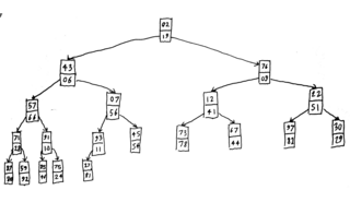
In computer science, the treap and the randomized binary search tree are two closely related forms of binary search tree data structures that maintain a dynamic set of ordered keys and allow binary searches among the keys. After any sequence of insertions and deletions of keys, the shape of the tree is a random variable with the same probability distribution as a random binary tree; in particular, with high probability its height is proportional to the logarithm of the number of keys, so that each search, insertion, or deletion operation takes logarithmic time to perform.

In computer science, a Fibonacci heap is a data structure for priority queue operations, consisting of a collection of heap-ordered trees. Fibonacci heaps were originally explained to be an extension of binomial queues. It has a better amortized running time than many other priority queue data structures including the binary heap and binomial heap. Michael L. Fredman and Robert E. Tarjan developed Fibonacci heaps in 1984 and published them in a scientific journal in 1987. Fibonacci heaps are named after the Fibonacci numbers, which are used in their running time analysis.

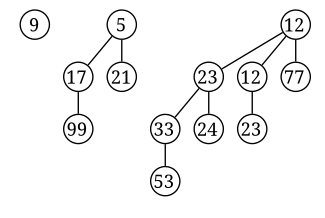
In computer science, a 2–3 heap is a data structure, a variation on the heap, designed by Tadao Takaoka in 1999. The structure is similar to the Fibonacci heap, and borrows from the 2–3 tree.

In computer science, a leftist tree or leftist heap is a priority queue implemented with a variant of a binary heap. Every node x has an s-value which is the distance to the nearest leaf in subtree rooted at x. In contrast to a binary heap, a leftist tree attempts to be very unbalanced. In addition to the heap property, leftist trees are maintained so the right descendant of each node has the lower s-value.

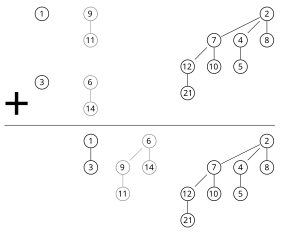
A pairing heap is a type of heap data structure with relatively simple implementation and excellent practical amortized performance, introduced by Michael Fredman, Robert Sedgewick, Daniel Sleator, and Robert Tarjan in 1986. Pairing heaps are heap-ordered multiway tree structures, and can be considered simplified Fibonacci heaps. They are considered a "robust choice" for implementing such algorithms as Prim's MST algorithm, and support the following operations :

The d-ary heap or d-heap is a priority queue data structure, a generalization of the binary heap in which the nodes have d children instead of 2. Thus, a binary heap is a 2-heap, and a ternary heap is a 3-heap. According to Tarjan and Jensen et al., d-ary heaps were invented by Donald B. Johnson in 1975.

<span class="mw-page-title-main">Cartesian tree</span> Binary tree derived from a sequence of numbers

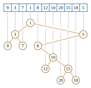
In computer science, a Cartesian tree is a binary tree derived from a sequence of distinct numbers. To construct the Cartesian tree, set its root to be the minimum number in the sequence, and recursively construct its left and right subtrees from the subsequences before and after this number. It is uniquely defined as a min-heap whose symmetric (in-order) traversal returns the original sequence.

In computer science, a min-max heap is a complete binary tree data structure which combines the usefulness of both a min-heap and a max-heap, that is, it provides constant time retrieval and logarithmic time removal of both the minimum and maximum elements in it. This makes the min-max heap a very useful data structure to implement a double-ended priority queue. Like binary min-heaps and max-heaps, min-max heaps support logarithmic insertion and deletion and can be built in linear time. Min-max heaps are often represented implicitly in an array; hence it's referred to as an implicit data structure.

In computer science, a skew binomial heap is a variant of the binomial heap that supports constant-time insertion operations in the worst case, rather than the logarithmic worst case and constant amortized time of ordinary binomial heaps. Just as binomial heaps are based on the binary number system, skew binary heaps are based on the skew binary number system.

In computer science, the Brodal queue is a heap/priority queue structure with very low worst case time bounds: for insertion, find-minimum, meld and decrease-key and for delete-minimum and general deletion. They are the first heap variant to achieve these bounds without resorting to amortization of operational costs. Brodal queues are named after their inventor Gerth Stølting Brodal.

In computer science, k-way merge algorithms or multiway merges are a specific type of sequence merge algorithms that specialize in taking in k sorted lists and merging them into a single sorted list. These merge algorithms generally refer to merge algorithms that take in a number of sorted lists greater than two. Two-way merges are also referred to as binary merges.The k- way merge is also an external sorting algorithm.

In computer science, a weak heap is a data structure for priority queues, combining features of the binary heap and binomial heap. It can be stored in an array as an implicit binary tree like a binary heap, and has the efficiency guarantees of binomial heaps.

<span class="mw-page-title-main">K-D heap</span>

A K-D heap is a data structure in computer science which implements a multidimensional priority queue without requiring additional space. It is a generalization of the Heap. It allows for efficient insertion, query of the minimum element, and deletion of the minimum element in any of the k dimensions, and therefore includes the double-ended heap as a special case.

This is a comparison of the performance of notable data structures, as measured by the complexity of their logical operations. For a more comprehensive listing of data structures, see List of data structures.

In computer science, a strict Fibonacci heap is a priority queue data structure with worst case time bounds equal to the amortized bounds of the Fibonacci heap. Strict Fibonacci heaps belong to a class of asymptotically optimal data structures for priority queues. All operations on strict Fibonacci heaps run in worst case constant time except delete-min, which is necessarily logarithmic. This is optimal, because any priority queue can be used to sort a list of elements by performing insertions and delete-min operations. Strict Fibonacci heaps were invented in 2012 by Gerth Stølting Brodal, George Lagogiannis, and Robert E. Tarjan.

References

  1. 1 2 3 4 5 6 7 8 9 10 11 12 13 14 15 16 17 Cormen, Thomas H.; Leiserson, Charles E.; Rivest, Ronald L.; Stein, Clifford (2001) [1990]. "Chapter 19: Binomial Heaps". Introduction to Algorithms (2nd ed.). MIT Press and McGraw-Hill. pp. 455–475. ISBN   0-262-03293-7.
  2. Vuillemin, Jean (1 April 1978). "A data structure for manipulating priority queues". Communications of the ACM. 21 (4): 309–315. doi: 10.1145/359460.359478 .
  3. 1 2 3 4 5 6 7 8 9 10 Brown, Mark R. (1978). "Implementation and analysis of binomial queue algorithms". SIAM Journal on Computing. 7 (3): 298–319. doi:10.1137/0207026. MR   0483830.
  4. Brodal, Gerth Stølting; Okasaki, Chris (November 1996), "Optimal purely functional priority queues", Journal of Functional Programming, 6 (6): 839–857, doi: 10.1017/s095679680000201x
  5. 1 2 3 4 Cormen, Thomas H.; Leiserson, Charles E.; Rivest, Ronald L. (1990). Introduction to Algorithms (1st ed.). MIT Press and McGraw-Hill. ISBN   0-262-03141-8.
  6. "Binomial Heap | Brilliant Math & Science Wiki". brilliant.org. Retrieved 30 September 2019.
  7. Brodal, Gerth Stølting; Okasaki, Chris (November 1996), "Optimal purely functional priority queues", Journal of Functional Programming, 6 (6): 839–857, doi: 10.1017/s095679680000201x
  8. Iacono, John (2000), "Improved upper bounds for pairing heaps", Proc. 7th Scandinavian Workshop on Algorithm Theory (PDF), Lecture Notes in Computer Science, vol. 1851, Springer-Verlag, pp. 63–77, arXiv: 1110.4428 , CiteSeerX   10.1.1.748.7812 , doi:10.1007/3-540-44985-X_5, ISBN   3-540-67690-2
  9. Fredman, Michael Lawrence (July 1999). "On the Efficiency of Pairing Heaps and Related Data Structures" (PDF). Journal of the Association for Computing Machinery . 46 (4): 473–501. doi:10.1145/320211.320214.
  10. Pettie, Seth (2005). Towards a Final Analysis of Pairing Heaps (PDF). FOCS '05 Proceedings of the 46th Annual IEEE Symposium on Foundations of Computer Science. pp. 174–183. CiteSeerX   10.1.1.549.471 . doi:10.1109/SFCS.2005.75. ISBN   0-7695-2468-0.
  11. Haeupler, Bernhard; Sen, Siddhartha; Tarjan, Robert E. (November 2011). "Rank-pairing heaps" (PDF). SIAM J. Computing. 40 (6): 1463–1485. doi:10.1137/100785351.
  12. Fredman, Michael Lawrence; Tarjan, Robert E. (July 1987). "Fibonacci heaps and their uses in improved network optimization algorithms" (PDF). Journal of the Association for Computing Machinery . 34 (3): 596–615. CiteSeerX   10.1.1.309.8927 . doi:10.1145/28869.28874.
  13. Brodal, Gerth Stølting; Lagogiannis, George; Tarjan, Robert E. (2012). Strict Fibonacci heaps (PDF). Proceedings of the 44th symposium on Theory of Computing - STOC '12. pp. 1177–1184. CiteSeerX   10.1.1.233.1740 . doi:10.1145/2213977.2214082. ISBN   978-1-4503-1245-5.
  14. Brodal, Gerth S. (1996), "Worst-Case Efficient Priority Queues" (PDF), Proc. 7th Annual ACM-SIAM Symposium on Discrete Algorithms, pp. 52–58
  15. Goodrich, Michael T.; Tamassia, Roberto (2004). "7.3.6. Bottom-Up Heap Construction". Data Structures and Algorithms in Java (3rd ed.). pp. 338–341. ISBN   0-471-46983-1.
  16. Takaoka, Tadao (1999), Theory of 2–3 Heaps (PDF), p. 12