Fibonacci heap

Fibonacci heap
Type	heap
Invented	1984
Invented by	Michael L. Fredman and Robert E. Tarjan
Complexities in big O notation
Space complexity Time complexity Function Amortized Worst Case Insert Θ(1) Find-min Θ(1) Delete-min O(log n) Decrease-key Θ(1) Merge Θ(1)

In computer science, a Fibonacci heap is a data structure for priority queue operations. It has a better amortized running time than many other priority queue data structures including the binary heap and binomial heap. consisting of a collection of heap-ordered trees. Michael L. Fredman and Robert E. Tarjan developed Fibonacci heaps in 1984 and published them in a scientific journal in 1987. Fibonacci heaps are named after the Fibonacci numbers, which are used in their running time analysis.

The amortized times of all operations on Fibonacci heaps is constant, except delete-min., the find-minimum operation takes constant amortized time. ^[1] The insert and decrease key operations also work in constant amortized time. ^[2] Deleting an element (most often used in the special case of deleting the minimum element) works in ${\displaystyle O(\log n)}$ amortized time, where ${\displaystyle n}$ is the size of the heap. ^[2] This means that starting from an empty data structure, any sequence of a insert and decrease-key operations and bdelete-min operations would take ${\displaystyle O(a+b\log n)}$ worst case time, where ${\displaystyle n}$ is the maximum heap size. In a binary or binomial heap, such a sequence of operations would take ${\displaystyle O((a+b)\log n)}$ time. A Fibonacci heap is thus better than a binary or binomial heap when ${\displaystyle b}$ is smaller than ${\displaystyle a}$ by a non-constant factor. It is also possible to merge two Fibonacci heaps in constant amortized time, improving on the logarithmic merge time of a binomial heap, and improving on binary heaps which cannot handle merges efficiently.

Using Fibonacci heaps for priority queues improves the asymptotic running time of important algorithms, such as Dijkstra's algorithm for computing the shortest path between two nodes in a graph, compared to the same algorithm using other slower priority queue data structures.

Structure

Figure 1. Example of a Fibonacci heap. It has three trees of degrees 0, 1 and 3. Three vertices are marked (shown in blue). Therefore, the potential of the heap is 9 (3 trees + 2 × (3 marked-vertices)).

A Fibonacci heap is a collection of trees satisfying the minimum-heap property, that is, the key of a child is always greater than or equal to the key of the parent. This implies that the minimum key is always at the root of one of the trees. Compared with binomial heaps, the structure of a Fibonacci heap is more flexible. The trees do not have a prescribed shape and in the extreme case the heap can have every element in a separate tree. This flexibility allows some operations to be executed in a lazy manner, postponing the work for later operations. For example, merging heaps is done simply by concatenating the two lists of trees, and operation decrease key sometimes cuts a node from its parent and forms a new tree.

However, at some point order needs to be introduced to the heap to achieve the desired running time. In particular, degrees of nodes (here degree means the number of direct children) are kept quite low: every node has degree at most ${\displaystyle \log n}$ and the size of a subtree rooted in a node of degree ${\displaystyle k}$ is at least ${\displaystyle F_{i+2}}$, where ${\displaystyle F_{i}}$ is the ${\displaystyle i}$th Fibonacci number. This is achieved by the rule: at most one child can be cut off each non-root node. When a second child is cut, the node itself needs to be cut from its parent and becomes the root of a new tree (see Proof of degree bounds, below). The number of trees is decreased in the operation delete-min, where trees are linked together.

As a result of a relaxed structure, some operations can take a long time while others are done very quickly. For the amortized running time analysis, we use the potential method, in that we pretend that very fast operations take a little bit longer than they actually do. This additional time is then later combined and subtracted from the actual running time of slow operations. The amount of time saved for later use is measured at any given moment by a potential function. The potential ${\displaystyle \phi }$ of a Fibonacci heap is given by

${\displaystyle \phi =t+2m}$,

where ${\displaystyle t}$ is the number of trees in the Fibonacci heap, and ${\displaystyle m}$ is the number of marked nodes. A node is marked if at least one of its children was cut, since this node was made a child of another node (all roots are unmarked). The amortized time for an operation is given by the sum of the actual time and ${\displaystyle c}$ times the difference in potential, where c is a constant (chosen to match the constant factors in the big O notation for the actual time).

Thus, the root of each tree in a heap has one unit of time stored. This unit of time can be used later to link this tree with another tree at amortized time 0. Also, each marked node has two units of time stored. One can be used to cut the node from its parent. If this happens, the node becomes a root and the second unit of time will remain stored in it as in any other root.

Operations

To allow fast deletion and concatenation, the roots of all trees are linked using a circular doubly linked list. The children of each node are also linked using such a list. For each node, we maintain its number of children and whether the node is marked.

Find-min

We maintain a pointer to the root containing the minimum key, allowing ${\displaystyle O(1)}$ access to the minimum. This pointer must be updated during the other operations, which adds only a constant time overhead.

Merge

The merge operation simply concatenates the root lists of two heaps together, and setting the minimum to be the smaller of the two heaps. This can be done in constant time, and the potential does not change, leading again to constant amortized time.

Insert

The insertion operation can be considered a special case of the merge operation, with a single node. The node is simply appended to the root list, increasing the potential by one. The amortized cost is thus still constant.

Delete-min

Figure 2. First phase of delete-min.

Figure 3. Third phase of delete-min.

The delete-min operation does most of the work in restoring the structure of the heap. It has three phases:

1. The root containing the minimum element is removed, and each of its ${\displaystyle d}$ children becomes a new root. It takes time ${\displaystyle O(d)}$ to process these new roots, and the potential increases by ${\displaystyle d-1}$. Therefore, the amortized running time of this phase is ${\displaystyle O(d)=O(\log n)}$.
2. There may be up to ${\displaystyle n}$ roots. We therefore decrease the number of roots by successively linking together roots of the same degree. When two roots have the same degree, we make the one with the larger key a child of the other, so that the minimum heap property is observed. The degree of the smaller root increases by one. This is repeated until every root has a different degree. To find trees of the same degree efficiently, we use an array of length ${\displaystyle O(\log n)}$ in which we keep a pointer to one root of each degree. When a second root is found of the same degree, the two are linked and the array is updated. The actual running time is ${\displaystyle O(\log n+m)}$, where ${\displaystyle m}$ is the number of roots at the beginning of the second phase. In the end, we will have at most ${\displaystyle O(\log n)}$ roots (because each has a different degree). Therefore, the difference in the potential from before to after this phase is ${\displaystyle O(\log n)-m}$. Thus, the amortized running time is ${\displaystyle O(\log n+m)+c(O(\log n)-m)}$. By choosing a sufficiently large ${\displaystyle c}$ such that the terms in ${\displaystyle m}$ cancel out, this simplifies to ${\displaystyle O(\log n)}$.
3. Search the final list of roots to find the minimum, and update the minimum pointer accordingly. This takes ${\displaystyle O(\log n)}$ time, because the number of roots has been reduced.

Overall, the amortized time of this operation is ${\displaystyle O(\log n)}$, provided that ${\displaystyle d=O(\log n)}$. The proof of this is given in the following section.

Decrease-key

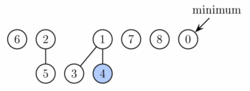
Figure 4. Fibonacci heap from Figure 1 after decreasing key of node 9 to 0.

If decreasing the key of a node ${\displaystyle x}$ causes it to become smaller than its parent, then it is cut from its parent, becoming a new unmarked root. If it is also less than the minimum key, then the minimum pointer is updated.

We then initiate a series of cascading cuts, starting with the parent of ${\displaystyle x}$. As long as the current node is marked, it is cut from its parent and made an unmarked root. Its original parent is then considered. This process stops when we reach an unmarked node ${\displaystyle y}$. If ${\displaystyle y}$ is not a root, it is marked. In this process we introduce some number, say ${\displaystyle k}$, of new trees. Except possibly ${\displaystyle x}$, each of these new trees was loses its original mark. The terminating node ${\displaystyle y}$ may become marked. Therefore, the change in the number of marked nodes is between of ${\displaystyle -k}$ and ${\displaystyle -k+2}$. The resulting change in potential is ${\displaystyle k+2(-k+2)=-k+4}$. The actual time required to perform the cutting was ${\displaystyle O(k)}$. Hence, the amortized time is ${\displaystyle O(k)+c(-k+4)}$, which is constant, provided ${\displaystyle c}$ is sufficiently large.

Proof of degree bounds

The amortized performance of a Fibonacci heap depends on the degree (number of children) of any tree root being ${\displaystyle O(\log n)}$, where ${\displaystyle n}$ is the size of the heap. Here we show that the size of the (sub)tree rooted at any node ${\displaystyle x}$ of degree ${\displaystyle d}$ in the heap must have size at least ${\displaystyle F_{d+2}}$, where ${\displaystyle F_{i}}$ is the ${\displaystyle i}$th Fibonacci number. The degree bound follows from this and the fact (easily proved by induction) that ${\displaystyle F_{d+2}\geq \varphi ^{d}}$ for all integers ${\displaystyle d\geq 0}$, where ${\displaystyle \varphi =(1+{\sqrt {5}})/2\approx 1.618}$ is the golden ratio. We then have ${\displaystyle n\geq F_{d+2}\geq \varphi ^{d}}$, and taking the log to base ${\displaystyle \varphi }$ of both sides gives ${\displaystyle d\leq \log _{\varphi }n}$ as required.

Let ${\displaystyle x}$ be an arbitrary node in a Fibonacci heap, not necessarily a root. Define ${\displaystyle \mathrm {size} (x)}$ to be the size of the tree rooted at ${\displaystyle x}$ (the number of descendants of ${\displaystyle x}$, including ${\displaystyle x}$ itself). We prove by induction on the height of ${\displaystyle x}$ (the length of the longest path from ${\displaystyle x}$ to a descendant leaf) that ${\displaystyle \mathrm {size} (x)\geq F_{d+2}}$, where ${\displaystyle d}$ is the degree of ${\displaystyle x}$.

Base case: If ${\displaystyle x}$ has height ${\displaystyle 0}$, then ${\displaystyle d=0}$, and ${\displaystyle \mathrm {size} (x)=1\geq F_{2}}$.

Inductive case: Suppose ${\displaystyle x}$ has positive height and degree ${\displaystyle d>0}$. Let ${\displaystyle y_{1},y_{2}\dots y_{d}}$ be the children of ${\displaystyle x}$, indexed in order of the times they were most recently made children of ${\displaystyle x}$ (${\displaystyle y_{1}}$ being the earliest and ${\displaystyle y_{d}}$ the latest), and let ${\displaystyle c_{1},c_{2}\dots c_{d}}$ be their respective degrees.

We claim that ${\displaystyle c_{i}\geq i-2}$ for each ${\displaystyle i}$. Just before ${\displaystyle y_{i}}$ was made a child of ${\displaystyle x}$, ${\displaystyle y_{1}\dots y_{i-1}}$ were already children of ${\displaystyle x}$, and so ${\displaystyle x}$ must have had degree at least ${\displaystyle i-1}$ at that time. Since trees are combined only when the degrees of their roots are equal, it must have been the case that ${\displaystyle y_{i}}$ also had degree at least ${\displaystyle i-1}$ at the time when it became a child of ${\displaystyle x}$. From that time to the present, ${\displaystyle y_{i}}$ could have only lost at most one child (as guaranteed by the marking process), and so its current degree ${\displaystyle c_{i}}$ is at least ${\displaystyle i-2}$. This proves the claim.

Since the heights of all the ${\displaystyle y_{i}}$ are strictly less than that of ${\displaystyle x}$, we can apply the inductive hypothesis to them to get

$${\displaystyle \mathrm {size} (y_{i})\geq F_{c_{i}+2}\geq F_{(i-2)+2}=F_{i}.}$$

The nodes ${\displaystyle x}$ and ${\displaystyle y_{1}}$ each contribute at least 1 to ${\displaystyle \mathrm {size} (x)}$, and so we have

$${\displaystyle {\begin{aligned}\mathrm {size} (x)&\geq 2+\sum _{i=2}^{d}\mathrm {size} (y_{i})\\&\geq 2+\sum _{i=2}^{d}F_{i}\\&=1+\sum _{i=0}^{d}F_{i}\\&=F_{d+2}\end{aligned}}}$$

where the last step is an identity for Fibonacci numbers. This gives the desired lower bound on ${\displaystyle \mathrm {size} (x)}$.

Performance

Although Fibonacci heaps look very efficient, they have the following two drawbacks: ^[3]

1. They are complicated to implement.
2. They are not as efficient in practice when compared with theoretically less efficient forms of heaps. ^[4] In their simplest version, they require manipulation of four pointers per node, whereas only two or three pointers per node are needed in other structures, such as the binomial heap, or pairing heap. This results in large memory consumption per node and high constant factors on all operations.

Although the total running time of a sequence of operations starting with an empty structure is bounded by the bounds given above, some (very few) operations in the sequence can take very long to complete (in particular, delete-min has linear running time in the worst case). For this reason, Fibonacci heaps and other amortized data structures may not be appropriate for real-time systems.

It is possible to create a data structure which has the same worst-case performance as the Fibonacci heap has amortized performance. One such structure, the Brodal queue, ^[5] is, in the words of the creator, "quite complicated" and "[not] applicable in practice." Invented in 2012, the strict Fibonacci heap ^[6] is a simpler (compared to Brodal's) structure with the same worst-case bounds. Despite being simpler, experiments show that in practice the strict Fibonacci heap performs slower than more complicated Brodal queue and also slower than basic Fibonacci heap. ^{[7] [8]} The run-relaxed heaps of Driscoll et al. give good worst-case performance for all Fibonacci heap operations except merge. ^[9] Recent experimental results suggest that the Fibonacci heap is more efficient in practice than most of its later derivatives, including quake heaps, violation heaps, strict Fibonacci heaps, and rank pairing heaps, but less efficient than pairing heaps or array-based heaps. ^[8]

Summary of running times

Here are time complexities ^[10] of various heap data structures. Function names assume a min-heap. For the meaning of "O(f)" and "Θ(f)" see Big O notation.

Operation	find-min	delete-min	insert	decrease-key	meld
Binary [10]	Θ(1)	Θ(log n)	O(log n)	O(log n)	Θ(n)
Leftist	Θ(1)	Θ(log n)	Θ(log n)	O(log n)	Θ(log n)
Binomial [10] [11]	Θ(1)	Θ(log n)	Θ(1) [lower-alpha 1]	Θ(log n)	O(log n)
Skew binomial [12]	Θ(1)	Θ(log n)	Θ(1)	Θ(log n)	O(log n) [lower-alpha 2]
Pairing [13]	Θ(1)	O(log n) [lower-alpha 1]	Θ(1)	o(log n) [lower-alpha 1] [lower-alpha 3]	Θ(1)
Rank-pairing [16]	Θ(1)	O(log n) [lower-alpha 1]	Θ(1)	Θ(1) [lower-alpha 1]	Θ(1)
Fibonacci [10] [2]	Θ(1)	O(log n) [lower-alpha 1]	Θ(1)	Θ(1) [lower-alpha 1]	Θ(1)
Strict Fibonacci [17]	Θ(1)	O(log n)	Θ(1)	Θ(1)	Θ(1)
Brodal [18] [lower-alpha 4]	Θ(1)	O(log n)	Θ(1)	Θ(1)	Θ(1)
2–3 heap [20]	O(log n)	O(log n) [lower-alpha 1]	O(log n) [lower-alpha 1]	Θ(1)	?

1. Amortized time.
2. Brodal and Okasaki describe a technique to reduce the worst-case complexity of meld to Θ(1); this technique applies to any heap datastructure that has insert in Θ(1) and find-min, delete-min, meld in O(log n).
3. Lower bound of ${\displaystyle \Omega (\log \log n),}$ ^[14] upper bound of ${\displaystyle O(2^{2{\sqrt {\log \log n}}}).}$ ^[15]
4. Brodal and Okasaki later describe a persistent variant with the same bounds except for decrease-key, which is not supported. Heaps with n elements can be constructed bottom-up in O(n). ^[19]

References

1. Cormen, Thomas H.; Leiserson, Charles E.; Rivest, Ronald L.; Stein, Clifford (2001) [1990]. "Chapter 20: Fibonacci Heaps". Introduction to Algorithms (2nd ed.). MIT Press and McGraw-Hill. pp. 476–497. ISBN   0-262-03293-7. Third edition p. 518.
2. Fredman, Michael Lawrence; Tarjan, Robert E. (July 1987). "Fibonacci heaps and their uses in improved network optimization algorithms" (PDF). Journal of the Association for Computing Machinery . 34 (3): 596–615. CiteSeerX   10.1.1.309.8927 . doi:10.1145/28869.28874.
3. Fredman, Michael L.; Sedgewick, Robert; Sleator, Daniel D.; Tarjan, Robert E. (1986). "The pairing heap: a new form of self-adjusting heap" (PDF). Algorithmica. 1 (1–4): 111–129. doi:10.1007/BF01840439. S2CID   23664143.
4. http://www.cs.princeton.edu/~wayne/kleinberg-tardos/pdf/FibonacciHeaps.pdf, p. 79
5. Gerth Stølting Brodal (1996), "Worst-Case Efficient Priority Queues", Proc. 7th ACM-SIAM Symposium on Discrete Algorithms, Society for Industrial and Applied Mathematics: 52–58, CiteSeerX   10.1.1.43.8133 , ISBN   0-89871-366-8
6. Brodal, G. S. L.; Lagogiannis, G.; Tarjan, R. E. (2012). Strict Fibonacci heaps (PDF). Proceedings of the 44th symposium on Theory of Computing - STOC '12. p. 1177. doi:10.1145/2213977.2214082. ISBN   978-1-4503-1245-5.
7. Mrena, Michal; Sedlacek, Peter; Kvassay, Miroslav (June 2019). "Practical Applicability of Advanced Implementations of Priority Queues in Finding Shortest Paths". 2019 International Conference on Information and Digital Technologies (IDT). Zilina, Slovakia: IEEE. pp. 335–344. doi:10.1109/DT.2019.8813457. ISBN   9781728114019. S2CID   201812705.
8. Larkin, Daniel; Sen, Siddhartha; Tarjan, Robert (2014). "A Back-to-Basics Empirical Study of Priority Queues". Proceedings of the Sixteenth Workshop on Algorithm Engineering and Experiments: 61–72. arXiv: 1403.0252 . Bibcode:2014arXiv1403.0252L. doi:10.1137/1.9781611973198.7. ISBN   978-1-61197-319-8. S2CID   15216766.
9. Driscoll, James R.; Gabow, Harold N.; Shrairman, Ruth; Tarjan, Robert E. (November 1988). "Relaxed heaps: An alternative to Fibonacci heaps with applications to parallel computation". Communications of the ACM. 31 (11): 1343–1354. doi: 10.1145/50087.50096 . S2CID   16078067.
10. Cormen, Thomas H.; Leiserson, Charles E.; Rivest, Ronald L. (1990). Introduction to Algorithms (1st ed.). MIT Press and McGraw-Hill. ISBN   0-262-03141-8.
11. "Binomial Heap | Brilliant Math & Science Wiki". brilliant.org. Retrieved 2019-09-30.
12. Brodal, Gerth Stølting; Okasaki, Chris (November 1996), "Optimal purely functional priority queues", Journal of Functional Programming, 6 (6): 839–857, doi: 10.1017/s095679680000201x
13. Iacono, John (2000), "Improved upper bounds for pairing heaps", Proc. 7th Scandinavian Workshop on Algorithm Theory (PDF), Lecture Notes in Computer Science, vol. 1851, Springer-Verlag, pp. 63–77, arXiv: 1110.4428 , CiteSeerX   10.1.1.748.7812 , doi:10.1007/3-540-44985-X_5, ISBN   3-540-67690-2
14. Fredman, Michael Lawrence (July 1999). "On the Efficiency of Pairing Heaps and Related Data Structures" (PDF). Journal of the Association for Computing Machinery . 46 (4): 473–501. doi:10.1145/320211.320214.
15. Pettie, Seth (2005). Towards a Final Analysis of Pairing Heaps (PDF). FOCS '05 Proceedings of the 46th Annual IEEE Symposium on Foundations of Computer Science. pp. 174–183. CiteSeerX   10.1.1.549.471 . doi:10.1109/SFCS.2005.75. ISBN   0-7695-2468-0.
16. Haeupler, Bernhard; Sen, Siddhartha; Tarjan, Robert E. (November 2011). "Rank-pairing heaps" (PDF). SIAM J. Computing. 40 (6): 1463–1485. doi:10.1137/100785351.
17. Brodal, Gerth Stølting; Lagogiannis, George; Tarjan, Robert E. (2012). Strict Fibonacci heaps (PDF). Proceedings of the 44th symposium on Theory of Computing - STOC '12. pp. 1177–1184. CiteSeerX   10.1.1.233.1740 . doi:10.1145/2213977.2214082. ISBN   978-1-4503-1245-5.
18. Brodal, Gerth S. (1996), "Worst-Case Efficient Priority Queues" (PDF), Proc. 7th Annual ACM-SIAM Symposium on Discrete Algorithms, pp. 52–58
19. Goodrich, Michael T.; Tamassia, Roberto (2004). "7.3.6. Bottom-Up Heap Construction". Data Structures and Algorithms in Java (3rd ed.). pp. 338–341. ISBN   0-471-46983-1.
20. Takaoka, Tadao (1999), Theory of 2–3 Heaps (PDF), p. 12

External links

• Java applet simulation of a Fibonacci heap
• MATLAB implementation of Fibonacci heap
• De-recursived and memory efficient C implementation of Fibonacci heap (free/libre software, CeCILL-B license)
• Ruby implementation of the Fibonacci heap (with tests)
• Pseudocode of the Fibonacci heap algorithm