The Navier–Stokes equations are partial differential equations which describe the motion of viscous fluid substances. They were named after French engineer and physicist Claude-Louis Navier and the Irish physicist and mathematician George Gabriel Stokes. They were developed over several decades of progressively building the theories, from 1822 (Navier) to 1842–1850 (Stokes).
The vorticity equation of fluid dynamics describes the evolution of the vorticity ω of a particle of a fluid as it moves with its flow; that is, the local rotation of the fluid. The governing equation is:
Linear elasticity is a mathematical model as to how solid objects deform and become internally stressed by prescribed loading conditions. It is a simplification of the more general nonlinear theory of elasticity and a branch of continuum mechanics.
In physics, the Hamilton–Jacobi equation, named after William Rowan Hamilton and Carl Gustav Jacob Jacobi, is an alternative formulation of classical mechanics, equivalent to other formulations such as Newton's laws of motion, Lagrangian mechanics and Hamiltonian mechanics.

Large eddy simulation (LES) is a mathematical model for turbulence used in computational fluid dynamics. It was initially proposed in 1963 by Joseph Smagorinsky to simulate atmospheric air currents, and first explored by Deardorff (1970). LES is currently applied in a wide variety of engineering applications, including combustion, acoustics, and simulations of the atmospheric boundary layer.

The Ekman layer is the layer in a fluid where there is a force balance between pressure gradient force, Coriolis force and turbulent drag. It was first described by Vagn Walfrid Ekman. Ekman layers occur both in the atmosphere and in the ocean.
In physics and fluid mechanics, a Blasius boundary layer describes the steady two-dimensional laminar boundary layer that forms on a semi-infinite plate which is held parallel to a constant unidirectional flow. Falkner and Skan later generalized Blasius' solution to wedge flow, i.e. flows in which the plate is not parallel to the flow.
The Mason–Weaver equation describes the sedimentation and diffusion of solutes under a uniform force, usually a gravitational field. Assuming that the gravitational field is aligned in the z direction, the Mason–Weaver equation may be written

Toroidal coordinates are a three-dimensional orthogonal coordinate system that results from rotating the two-dimensional bipolar coordinate system about the axis that separates its two foci. Thus, the two foci and in bipolar coordinates become a ring of radius in the plane of the toroidal coordinate system; the -axis is the axis of rotation. The focal ring is also known as the reference circle.
Prolate spheroidal coordinates are a three-dimensional orthogonal coordinate system that results from rotating the two-dimensional elliptic coordinate system about the focal axis of the ellipse, i.e., the symmetry axis on which the foci are located. Rotation about the other axis produces oblate spheroidal coordinates. Prolate spheroidal coordinates can also be considered as a limiting case of ellipsoidal coordinates in which the two smallest principal axes are equal in length.

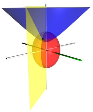
Oblate spheroidal coordinates are a three-dimensional orthogonal coordinate system that results from rotating the two-dimensional elliptic coordinate system about the non-focal axis of the ellipse, i.e., the symmetry axis that separates the foci. Thus, the two foci are transformed into a ring of radius in the x-y plane. Oblate spheroidal coordinates can also be considered as a limiting case of ellipsoidal coordinates in which the two largest semi-axes are equal in length.
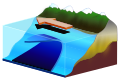
Ekman transport is part of Ekman motion theory, first investigated in 1902 by Vagn Walfrid Ekman. Winds are the main source of energy for ocean circulation, and Ekman transport is a component of wind-driven ocean current. Ekman transport occurs when ocean surface waters are influenced by the friction force acting on them via the wind. As the wind blows it casts a friction force on the ocean surface that drags the upper 10-100m of the water column with it. However, due to the influence of the Coriolis effect, the ocean water moves at a 90° angle from the direction of the surface wind. The direction of transport is dependent on the hemisphere: in the northern hemisphere, transport occurs at 90° clockwise from wind direction, while in the southern hemisphere it occurs at 90° anticlockwise. This phenomenon was first noted by Fridtjof Nansen, who recorded that ice transport appeared to occur at an angle to the wind direction during his Arctic expedition of the 1890s. Ekman transport has significant impacts on the biogeochemical properties of the world's oceans. This is because it leads to upwelling and downwelling in order to obey mass conservation laws. Mass conservation, in reference to Ekman transfer, requires that any water displaced within an area must be replenished. This can be done by either Ekman suction or Ekman pumping depending on wind patterns.
The derivation of the Navier–Stokes equations as well as their application and formulation for different families of fluids, is an important exercise in fluid dynamics with applications in mechanical engineering, physics, chemistry, heat transfer, and electrical engineering. A proof explaining the properties and bounds of the equations, such as Navier–Stokes existence and smoothness, is one of the important unsolved problems in mathematics.
In physical oceanography and fluid dynamics, the wind stress is the shear stress exerted by the wind on the surface of large bodies of water – such as oceans, seas, estuaries and lakes. When wind is blowing over a water surface, the wind applies a wind force on the water surface. The wind stress is the component of this wind force that is parallel to the surface per unit area. Also, the wind stress can be described as the flux of horizontal momentum applied by the wind on the water surface. The wind stress causes a deformation of the water body whereby wind waves are generated. Also, the wind stress drives ocean currents and is therefore an important driver of the large-scale ocean circulation. The wind stress is affected by the wind speed, the shape of the wind waves and the atmospheric stratification. It is one of the components of the air–sea interaction, with others being the atmospheric pressure on the water surface, as well as the exchange of energy and mass between the water and the atmosphere.
The Cauchy momentum equation is a vector partial differential equation put forth by Cauchy that describes the non-relativistic momentum transport in any continuum.
Shear velocity, also called friction velocity, is a form by which a shear stress may be re-written in units of velocity. It is useful as a method in fluid mechanics to compare true velocities, such as the velocity of a flow in a stream, to a velocity that relates shear between layers of flow.
In fluid dynamics, the Oseen equations describe the flow of a viscous and incompressible fluid at small Reynolds numbers, as formulated by Carl Wilhelm Oseen in 1910. Oseen flow is an improved description of these flows, as compared to Stokes flow, with the (partial) inclusion of convective acceleration.
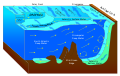
Ocean dynamics define and describe the flow of water within the oceans. Ocean temperature and motion fields can be separated into three distinct layers: mixed (surface) layer, upper ocean, and deep ocean.
Von Kármán swirling flow is a flow created by a uniformly rotating infinitely long plane disk, named after Theodore von Kármán who solved the problem in 1921. The rotating disk acts as a fluid pump and is used as a model for centrifugal fans or compressors. This flow is classified under the category of steady flows in which vorticity generated at a solid surface is prevented from diffusing far away by an opposing convection, the other examples being the Blasius boundary layer with suction, stagnation point flow etc.
Ball divergence is a non-parametric two-sample statistical test method in metric spaces. It measures the difference between two population probability distributions by integrating the difference over all balls in the space. Therefore, its value is zero if and only if the two probability measures are the same. Similar to common non-parametric test methods, ball divergence calculates the p-value through permutation tests.