Airy wave theory

Last updated

In fluid dynamics, Airy wave theory (often referred to as linear wave theory) gives a linearised description of the propagation of gravity waves on the surface of a homogeneous fluid layer. The theory assumes that the fluid layer has a uniform mean depth, and that the fluid flow is inviscid, incompressible and irrotational. This theory was first published, in correct form, by George Biddell Airy in the 19th century. [1]

Contents

Airy wave theory is often applied in ocean engineering and coastal engineering for the modelling of random sea states – giving a description of the wave kinematics and dynamics of high-enough accuracy for many purposes. [2] [3] Further, several second-order nonlinear properties of surface gravity waves, and their propagation, can be estimated from its results. [4] Airy wave theory is also a good approximation for tsunami waves in the ocean, before they steepen near the coast.

This linear theory is often used to get a quick and rough estimate of wave characteristics and their effects. This approximation is accurate for small ratios of the wave height to water depth (for waves in shallow water), and wave height to wavelength (for waves in deep water).

Description

Wave characteristics. Sine wave amplitude.svg
Wave characteristics.
Dispersion of gravity waves on a fluid surface. Phase and group velocity divided by [?]gh as a function of
.mw-parser-output .sfrac{white-space:nowrap}.mw-parser-output .sfrac.tion,.mw-parser-output .sfrac .tion{display:inline-block;vertical-align:-0.5em;font-size:85%;text-align:center}.mw-parser-output .sfrac .num{display:block;line-height:1em;margin:0.0em 0.1em;border-bottom:1px solid}.mw-parser-output .sfrac .den{display:block;line-height:1em;margin:0.1em 0.1em}.mw-parser-output .sr-only{border:0;clip:rect(0,0,0,0);clip-path:polygon(0px 0px,0px 0px,0px 0px);height:1px;margin:-1px;overflow:hidden;padding:0;position:absolute;width:1px}
h/l. A: phase velocity, B: group velocity, C: phase and group velocity [?]gh valid in shallow water. Drawn lines: based on dispersion relation valid in arbitrary depth. Dashed lines: based on dispersion relation valid in deep water. Dispersion gravity 1.svg
Dispersion of gravity waves on a fluid surface. Phase and group velocity divided by gh as a function of h/λ. A: phase velocity, B: group velocity, C: phase and group velocity gh valid in shallow water. Drawn lines: based on dispersion relation valid in arbitrary depth. Dashed lines: based on dispersion relation valid in deep water.

Airy wave theory uses a potential flow (or velocity potential) approach to describe the motion of gravity waves on a fluid surface. The use of (inviscid and irrotational) potential flow in water waves is remarkably successful, given its failure to describe many other fluid flows where it is often essential to take viscosity, vorticity, turbulence or flow separation into account. This is due to the fact that for the oscillatory part of the fluid motion, wave-induced vorticity is restricted to some thin oscillatory Stokes boundary layers at the boundaries of the fluid domain. [5]

Airy wave theory is often used in ocean engineering and coastal engineering. Especially for random waves, sometimes called wave turbulence, the evolution of the wave statistics – including the wave spectrum – is predicted well over not too long distances (in terms of wavelengths) and in not too shallow water. Diffraction is one of the wave effects which can be described with Airy wave theory. Further, by using the WKBJ approximation, wave shoaling and refraction can be predicted. [2]

Earlier attempts to describe surface gravity waves using potential flow were made by, among others, Laplace, Poisson, Cauchy and Kelland. But Airy was the first to publish the correct derivation and formulation in 1841. [1] Soon after, in 1847, the linear theory of Airy was extended by Stokes for non-linear wave motion – known as Stokes' wave theory – correct up to third order in the wave steepness. [6] Even before Airy's linear theory, Gerstner derived a nonlinear trochoidal wave theory in 1802, which however is not irrotational. [1]

Airy wave theory is a linear theory for the propagation of waves on the surface of a potential flow and above a horizontal bottom. The free surface elevation η(x,t) of one wave component is sinusoidal, as a function of horizontal position x and time t:

where

The waves propagate along the water surface with the phase speed cp:

The angular wavenumber k and frequency ω are not independent parameters (and thus also wavelength λ and period T are not independent), but are coupled. Surface gravity waves on a fluid are dispersive waves – exhibiting frequency dispersion – meaning that each wavenumber has its own frequency and phase speed.

Note that in engineering the wave height H – the difference in elevation between crest and trough – is often used:

valid in the present case of linear periodic waves.

Orbital motion under linear waves. The yellow dots indicate the momentary position of fluid particles on their (orange) orbits. The black dots are the centres of the orbits. Orbital wave motion.svg
Orbital motion under linear waves. The yellow dots indicate the momentary position of fluid particles on their (orange) orbits. The black dots are the centres of the orbits.
Particle motion in an ocean wave at deep (A) and shallow (B) depths. 1) Propagation direction. 2) Wave crest. 3) Wave trough. Wave motion-i18n-mod-with-ground.svg
Particle motion in an ocean wave at deep (A) and shallow (B) depths. 1) Propagation direction. 2) Wave crest. 3) Wave trough.

Underneath the surface, there is a fluid motion associated with the free surface motion. While the surface elevation shows a propagating wave, the fluid particles are in an orbital motion. Within the framework of Airy wave theory, the orbits are closed curves: circles in deep water and ellipses in finite depth—with the circles dying out before reaching the bottom of the fluid layer, and the ellipses becoming flatter near the bottom of the fluid layer. So while the wave propagates, the fluid particles just orbit (oscillate) around their average position. With the propagating wave motion, the fluid particles transfer energy in the wave propagation direction, without having a mean velocity. The diameter of the orbits reduces with depth below the free surface. In deep water, the orbit's diameter is reduced to 4% of its free-surface value at a depth of half a wavelength.

In a similar fashion, there is also a pressure oscillation underneath the free surface, with wave-induced pressure oscillations reducing with depth below the free surface – in the same way as for the orbital motion of fluid parcels.

Mathematical formulation of the wave motion

Flow problem formulation

The waves propagate in the horizontal direction, with coordinate x, and a fluid domain bound above by a free surface at z = η(x,t), with z the vertical coordinate (positive in the upward direction) and t being time. [7] The level z = 0 corresponds with the mean surface elevation. The impermeable bed underneath the fluid layer is at z = −h. Further, the flow is assumed to be incompressible and irrotational – a good approximation of the flow in the fluid interior for waves on a liquid surface – and potential theory can be used to describe the flow. The velocity potential Φ(x, z, t) is related to the flow velocity components ux and uz in the horizontal (x) and vertical (z) directions by:

Then, due to the continuity equation for an incompressible flow, the potential Φ has to satisfy the Laplace equation:

Boundary conditions are needed at the bed and the free surface in order to close the system of equations. For their formulation within the framework of linear theory, it is necessary to specify what the base state (or zeroth-order solution) of the flow is. Here, we assume the base state is rest, implying the mean flow velocities are zero.

The bed being impermeable, leads to the kinematic bed boundary-condition:

In case of deep water – by which is meant infinite water depth, from a mathematical point of view – the flow velocities have to go to zero in the limit as the vertical coordinate goes to minus infinity: z → −∞.

At the free surface, for infinitesimal waves, the vertical motion of the flow has to be equal to the vertical velocity of the free surface. This leads to the kinematic free-surface boundary-condition:

If the free surface elevation η(x,t) was a known function, this would be enough to solve the flow problem. However, the surface elevation is an extra unknown, for which an additional boundary condition is needed. This is provided by Bernoulli's equation for an unsteady potential flow. The pressure above the free surface is assumed to be constant. This constant pressure is taken equal to zero, without loss of generality, since the level of such a constant pressure does not alter the flow. After linearisation, this gives the dynamic free-surface boundary condition:

Because this is a linear theory, in both free-surface boundary conditions – the kinematic and the dynamic one, equations ( 3 ) and ( 4 ) – the value of Φ and ∂Φ/z at the fixed mean level z = 0 is used.

Solution for a progressive monochromatic wave

For a propagating wave of a single frequency – a monochromatic wave – the surface elevation is of the form: [7]

The associated velocity potential, satisfying the Laplace equation (1) in the fluid interior, as well as the kinematic boundary conditions at the free surface (2), and bed (3), is:

with sinh and cosh the hyperbolic sine and hyperbolic cosine function, respectively. But η and Φ also have to satisfy the dynamic boundary condition, which results in non-trivial (non-zero) values for the wave amplitude a only if the linear dispersion relation is satisfied:

with tanh the hyperbolic tangent. So angular frequency ω and wavenumber k – or equivalently period T and wavelength λ – cannot be chosen independently, but are related. This means that wave propagation at a fluid surface is an eigenproblem. When ω and k satisfy the dispersion relation, the wave amplitude a can be chosen freely (but small enough for Airy wave theory to be a valid approximation).

Table of wave quantities

In the table below, several flow quantities and parameters according to Airy wave theory are given. [7] The given quantities are for a bit more general situation as for the solution given above. Firstly, the waves may propagate in an arbitrary horizontal direction in the x = (x,y) plane. The wavenumber vector is k, and is perpendicular to the cams of the wave crests. Secondly, allowance is made for a mean flow velocity U, in the horizontal direction and uniform over (independent of) depth z. This introduces a Doppler shift in the dispersion relations. At an Earth-fixed location, the observed angular frequency (or absolute angular frequency) is ω. On the other hand, in a frame of reference moving with the mean velocity U (so the mean velocity as observed from this reference frame is zero), the angular frequency is different. It is called the intrinsic angular frequency (or relative angular frequency), denoted σ. So in pure wave motion, with U = 0, both frequencies ω and σ are equal. The wave number k (and wavelength λ) are independent of the frame of reference, and have no Doppler shift (for monochromatic waves).

The table only gives the oscillatory parts of flow quantities – velocities, particle excursions and pressure – and not their mean value or drift. The oscillatory particle excursions ξx and ξz are the time integrals of the oscillatory flow velocities ux and uz respectively.

Water depth is classified into three regimes: [8]

Visualization of deep and shallow water waves by relating wavelength to depth to bed. Deep and shallow water waves.pdf
Visualization of deep and shallow water waves by relating wavelength to depth to bed.

In the limiting cases of deep and shallow water, simplifying approximations to the solution can be made. While for intermediate depth, the full formulations have to be used.

Properties of gravity waves on the surface of deep water, shallow water and at intermediate depth, according to Airy wave theory [7]
quantitysymbolunitsdeep water
(h > 1/2λ)
shallow water
(h < 1/20λ)
intermediate depth
(all λ and h)
surface elevationm
wave phase rad
observed angular frequency rad·s −1
intrinsic angular frequencyrad·s −1
unit vector in the wave propagation direction
dispersion relation rad·s −1
phase speed m·s−1
group speed m·s−1
ratio
horizontal velocitym·s−1
vertical velocitym·s−1
horizontal particle excursionm
vertical particle excursionm
pressure oscillation N·m−2

Surface tension effects

Dispersion of gravity-capillary waves on the surface of deep water. Phase and group velocity divided by [?]gs / r as a function of inverse relative wavelength
1/l[?]s / rg.
Blue lines (A): phase velocity cp, Red lines (B): group velocity cg.
Drawn lines: gravity-capillary waves.
Dashed lines: gravity waves.
Dash-dot lines: pure capillary waves.
Note: s is surface tension in this graph. Dispersion capillary.svg
Dispersion of gravity–capillary waves on the surface of deep water. Phase and group velocity divided by / ρ as a function of inverse relative wavelength 1/λσ / ρg.
Blue lines (A): phase velocity cp, Red lines (B): group velocity cg.
Drawn lines: gravity–capillary waves.
Dashed lines: gravity waves.
Dash-dot lines: pure capillary waves.
Note: σ is surface tension in this graph.

Due to surface tension, the dispersion relation changes to: [11]

with γ the surface tension in newtons per metre. All above equations for linear waves remain the same, if the gravitational acceleration g is replaced by [12]

As a result of surface tension, the waves propagate faster. Surface tension only has influence for short waves, with wavelengths less than a few decimeters in case of a water–air interface. For very short wavelengths – 2 mm or less, in case of the interface between air and water – gravity effects are negligible. Note that surface tension can be altered by surfactants.

The group velocity ∂Ω/k of capillary waves – dominated by surface tension effects – is greater than the phase velocity Ω/k. This is opposite to the situation of surface gravity waves (with surface tension negligible compared to the effects of gravity) where the phase velocity exceeds the group velocity. [13]

Interfacial waves

Surface waves are a special case of interfacial waves, on the interface between two fluids of different density.

Two layers of infinite depth

Consider two fluids separated by an interface, and without further boundaries. Then their dispersion relation ω2 = Ω2(k) is given through [11] [14] [15]

where ρ and ρ are the densities of the two fluids, below (ρ) and above (ρ) the interface, respectively. Further γ is the surface tension on the interface.

For interfacial waves to exist, the lower layer has to be heavier than the upper one, ρ > ρ. Otherwise, the interface is unstable and a Rayleigh–Taylor instability develops.

Two layers between horizontal rigid planes

Wave motion on the interface between two layers of inviscid homogeneous fluids of different density, confined between horizontal rigid boundaries (at the top and bottom). The motion is forced by gravity. The upper layer has mean depth h' and density r', while the lower layer has mean depth h and density r. The wave amplitude is a, the wavelength is denoted by l (related to the wavenumber k by k =
2p/l), the gravitational acceleration by g and the phase speed by cp (with cp =
O(k)/k). Interfacial wave rigid boundaries.svg
Wave motion on the interface between two layers of inviscid homogeneous fluids of different density, confined between horizontal rigid boundaries (at the top and bottom). The motion is forced by gravity. The upper layer has mean depth h and density ρ, while the lower layer has mean depth h and density ρ. The wave amplitude is a, the wavelength is denoted by λ (related to the wavenumber k by k = 2π/λ), the gravitational acceleration by g and the phase speed by cp (with cp = Ω(k)/k).

For two homogeneous layers of fluids, of mean thickness h below the interface and h above – under the action of gravity and bounded above and below by horizontal rigid walls – the dispersion relationship ω2 = Ω2(k) for gravity waves is provided by: [16]

where again ρ and ρ are the densities below and above the interface, while coth is the hyperbolic cotangent function. For the case ρ is zero this reduces to the dispersion relation of surface gravity waves on water of finite depth h.

Two layers bounded above by a free surface

In this case the dispersion relation allows for two modes: a barotropic mode where the free surface amplitude is large compared with the amplitude of the interfacial wave, and a baroclinic mode where the opposite is the case – the interfacial wave is higher than and in antiphase with the free surface wave. The dispersion relation for this case is of a more complicated form. [17]

Second-order wave properties

Several second-order wave properties, ones that are quadratic in the wave amplitude a, can be derived directly from Airy wave theory. They are of importance in many practical applications, such as forecasts of wave conditions. [18] Using a WKBJ approximation, second-order wave properties also find their applications in describing waves in case of slowly varying bathymetry, and mean-flow variations of currents and surface elevation. As well as in the description of the wave and mean-flow interactions due to time and space-variations in amplitude, frequency, wavelength and direction of the wave field itself.

Table of second-order wave properties

In the table below, several second-order wave properties – as well as the dynamical equations they satisfy in case of slowly varying conditions in space and time – are given. More details on these can be found below. The table gives results for wave propagation in one horizontal spatial dimension. Further on in this section, more detailed descriptions and results are given for the general case of propagation in two-dimensional horizontal space.

Second-order quantities and their dynamics, using results of Airy wave theory
quantitysymbolunitsformula
mean wave-energy density per unit horizontal area J·m−2
radiation stress or excess horizontal momentum flux due to the wave motionN·m−1
wave action J·s·m−2
mean mass-flux due to the wave motion or the wave pseudo-momentumkg·m−1·s−1
mean horizontal mass-transport velocitym·s−1
Stokes drift m·s−1
wave-energy propagationJ·m−2·s−1
wave action conservationJ·m−2
wave-crest conservationrad·m−1·s−1
mean mass conservationkg·m−2·s−1
mean horizontal-momentum evolutionN·m−2

The last four equations describe the evolution of slowly varying wave trains over bathymetry in interaction with the mean flow, and can be derived from a variational principle: Whitham's averaged Lagrangian method. [19] In the mean horizontal-momentum equation, d(x) is the still water depth, that is, the bed underneath the fluid layer is located at z = −d. Note that the mean-flow velocity in the mass and momentum equations is the mass transport velocityŨ, including the splash-zone effects of the waves on horizontal mass transport, and not the mean Eulerian velocity (for example, as measured with a fixed flow meter).

Wave energy density

Wave energy is a quantity of primary interest, since it is a primary quantity that is transported with the wave trains. [20] As can be seen above, many wave quantities like surface elevation and orbital velocity are oscillatory in nature with zero mean (within the framework of linear theory). In water waves, the most used energy measure is the mean wave energy density per unit horizontal area. It is the sum of the kinetic and potential energy density, integrated over the depth of the fluid layer and averaged over the wave phase. Simplest to derive is the mean potential energy density per unit horizontal area Epot of the surface gravity waves, which is the deviation of the potential energy due to the presence of the waves: [21]

The overbar denotes the mean value (which in the present case of periodic waves can be taken either as a time average or an average over one wavelength in space).

The mean kinetic energy density per unit horizontal area Ekin of the wave motion is similarly found to be: [21]

with σ the intrinsic frequency, see the table of wave quantities. Using the dispersion relation, the result for surface gravity waves is:

As can be seen, the mean kinetic and potential energy densities are equal. This is a general property of energy densities of progressive linear waves in a conservative system. [22] [23] Adding potential and kinetic contributions, Epot and Ekin, the mean energy density per unit horizontal area E of the wave motion is:

In case of surface tension effects not being negligible, their contribution also adds to the potential and kinetic energy densities, giving [22]

so

with γ the surface tension.

Wave action, wave energy flux and radiation stress

In general, there can be an energy transfer between the wave motion and the mean fluid motion. This means, that the wave energy density is not in all cases a conserved quantity (neglecting dissipative effects), but the total energy density – the sum of the energy density per unit area of the wave motion and the mean flow motion – is. However, there is for slowly varying wave trains, propagating in slowly varying bathymetry and mean-flow fields, a similar and conserved wave quantity, the wave action A = E/σ: [19] [24] [25]

with (U + cg) A the action flux and cg = cgek the group velocity vector. Action conservation forms the basis for many wind wave models and wave turbulence models. [26] It is also the basis of coastal engineering models for the computation of wave shoaling. [27] Expanding the above wave action conservation equation leads to the following evolution equation for the wave energy density: [28]

with:

In this equation in non-conservation form, the Frobenius inner product S : (∇U) is the source term describing the energy exchange of the wave motion with the mean flow. Only in the case that the mean shear-rate is zero, U = 0, the mean wave energy density E is conserved. The two tensors S and U are in a Cartesian coordinate system of the form: [29]

with kx and ky the components of the wavenumber vector k and similarly Ux and Uy the components in of the mean velocity vector U.

Wave mass flux and wave momentum

The mean horizontal momentum per unit area M induced by the wave motion – and also the wave-induced mass flux or mass transport – is: [30]

which is an exact result for periodic progressive water waves, also valid for nonlinear waves. [31] However, its validity strongly depends on the way how wave momentum and mass flux are defined. Stokes already identified two possible definitions of phase velocity for periodic nonlinear waves: [6]

The above relation between wave momentum M and wave energy density E is valid within the framework of Stokes' first definition.

However, for waves perpendicular to a coast line or in closed laboratory wave channel, the second definition (S2) is more appropriate. These wave systems have zero mass flux and momentum when using the second definition. [32] In contrast, according to Stokes' first definition (S1), there is a wave-induced mass flux in the wave propagation direction, which has to be balanced by a mean flow U in the opposite direction – called the undertow.

So in general, there are quite some subtleties involved. Therefore also the term pseudo-momentum of the waves is used instead of wave momentum. [33]

Mass and momentum evolution equations

For slowly varying bathymetry, wave and mean-flow fields, the evolution of the mean flow can de described in terms of the mean mass-transport velocity Ũ defined as: [34]

Note that for deep water, when the mean depth h goes to infinity, the mean Eulerian velocity U and mean transport velocity Ũ become equal.

The equation for mass conservation is: [19] [34]

where h(x,t) is the mean water depth, slowly varying in space and time.

Similarly, the mean horizontal momentum evolves as: [19] [34]

with d the still-water depth (the sea bed is at z = –d), S is the wave radiation-stress tensor, I is the identity matrix and is the dyadic product:

Note that mean horizontal momentum is only conserved if the sea bed is horizontal (the still-water depth d is a constant), in agreement with Noether's theorem.

The system of equations is closed through the description of the waves. Wave energy propagation is described through the wave-action conservation equation (without dissipation and nonlinear wave interactions): [19] [24]

The wave kinematics are described through the wave-crest conservation equation: [35]

with the angular frequency ω a function of the (angular) wavenumber k, related through the dispersion relation. For this to be possible, the wave field must be coherent. By taking the curl of the wave-crest conservation, it can be seen that an initially irrotational wavenumber field stays irrotational.

Stokes drift

When following a single particle in pure wave motion (U = 0), according to linear Airy wave theory, a first approximation gives closed elliptical orbits for water particles. [36] However, for nonlinear waves, particles exhibit a Stokes drift for which a second-order expression can be derived from the results of Airy wave theory (see the table above on second-order wave properties). [37] The Stokes drift velocity ūS, which is the particle drift after one wave cycle divided by the period, can be estimated using the results of linear theory: [38]

so it varies as a function of elevation. The given formula is for Stokes first definition of wave celerity. When ρūS is integrated over depth, the expression for the mean wave momentum M is recovered. [38]

See also

Notes

  1. 1 2 3 Craik (2004).
  2. 1 2 Goda, Y. (2000). Random Seas and Design of Maritime Structures. Advanced Series on Ocean Engineering. Vol. 15. Singapore: World Scientific Publishing Company. ISBN   978-981-02-3256-6. OCLC   45200228.
  3. Dean & Dalrymple (1991).
  4. Phillips (1977), §3.2, pp. 37–43 and §3.6, pp. 60–69.
  5. Lighthill, M. J. (1986). "Fundamentals concerning wave loading on offshore structures". J. Fluid Mech. 173: 667–681. Bibcode:1986JFM...173..667L. doi:10.1017/S0022112086001313. S2CID   113694460.
  6. 1 2 Stokes (1847).
  7. 1 2 3 4 For the equations, solution and resulting approximations in deep and shallow water, see Dingemans (1997), Part 1, §2.1, pp. 38–45. Or: Phillips (1977), pp. 36–45.
  8. Dean & Dalrymple (1991) pp. 64–65
  9. The error in the phase speed is less than 0.2% if depth h is taken to be infinite, for h > 1/2λ.
  10. The error in the phase speed is less than 2% if wavelength effects are neglected for h < 1/20λ.
  11. 1 2 Phillips (1977), p. 37.
  12. Lighthill (1978), p. 223.
  13. Phillips (1977), p. 175.
  14. Lamb, H. (1994), §267, page 458–460.
  15. Dingemans (1997), Section 2.1.1, p. 45.
  16. Turner, J. S. (1979), Buoyancy effects in fluids, Cambridge University Press, p. 18, ISBN   978-0521297264
  17. Apel, J. R. (1987), Principles of ocean physics, Academic Press, pp. 231–239, ISBN   9780080570747
  18. See for example: the High seas forecasts of NOAA's National Weather service.
  19. 1 2 3 4 5 Whitham, G.B. (1974). Linear and nonlinear waves. Wiley-Interscience. ISBN   978-0-471-94090-6. OCLC   815118., p. 559.
  20. Phillips (1977), p. 23–25.
  21. 1 2 Phillips (1977), p. 39.
  22. 1 2 Phillips (1977), p. 38.
  23. Lord Rayleigh (J. W. Strutt) (1877). "On progressive waves". Proceedings of the London Mathematical Society. 9: 21–26. doi:10.1112/plms/s1-9.1.21. Reprinted as Appendix in: Theory of Sound1, MacMillan, 2nd revised edition, 1894.
  24. 1 2 Phillips (1977), p. 26.
  25. Bretherton, F. P.; Garrett, C. J. R. (1968). "Wavetrains in inhomogeneous moving media". Proceedings of the Royal Society of London, Series A. 302 (1471): 529–554. Bibcode:1968RSPSA.302..529B. doi:10.1098/rspa.1968.0034. S2CID   202575349.
  26. Phillips (1977), pp. 179–183.
  27. Phillips (1977), pp. 70–74.
  28. Phillips (1977), p. 66.
  29. Phillips (1977), p. 68.
  30. Phillips (1977), pp. 39–40 & 61.
  31. Phillips (1977), p. 40.
  32. Phillips (1977), p. 70.
  33. McIntyre, M. E. (1978). "On the 'wave-momentum' myth". Journal of Fluid Mechanics. 106: 331–347. Bibcode:1981JFM...106..331M. doi:10.1017/S0022112081001626. S2CID   18232994.
  34. 1 2 3 Phillips (1977), pp. 61–63.
  35. Phillips (1977), p. 23.
  36. LeBlond, P.H.; Mysak, L.A. (1981). Waves in the Ocean. Elsevier Oceanography Series. Vol. 20. Elsevier. pp. 85 & 110–111. ISBN   978-0-444-41926-2.
  37. Craik, A.D.D. (1988). Wave interactions and fluid flows. Cambridge University Press. p. 105. ISBN   978-0-521-36829-2.
  38. 1 2 Phillips (1977), p. 44.

Related Research Articles

<span class="mw-page-title-main">Navier–Stokes equations</span> Equations describing the motion of viscous fluid substances

The Navier–Stokes equations are partial differential equations which describe the motion of viscous fluid substances. They were named after French engineer and physicist Claude-Louis Navier and the Irish physicist and mathematician George Gabriel Stokes. They were developed over several decades of progressively building the theories, from 1822 (Navier) to 1842–1850 (Stokes).

<span class="mw-page-title-main">Potential flow</span> Velocity field as the gradient of a scalar function

In fluid dynamics, potential flow or irrotational flow refers to a description of a fluid flow with no vorticity in it. Such a description typically arises in the limit of vanishing viscosity, i.e., for an inviscid fluid and with no vorticity present in the flow.

<span class="mw-page-title-main">Gravity wave</span> Wave in or at the interface between fluids where gravity is the main equilibrium force

In fluid dynamics, gravity waves are waves generated in a fluid medium or at the interface between two media when the force of gravity or buoyancy tries to restore equilibrium. An example of such an interface is that between the atmosphere and the ocean, which gives rise to wind waves.

The vorticity equation of fluid dynamics describes the evolution of the vorticity ω of a particle of a fluid as it moves with its flow; that is, the local rotation of the fluid. The governing equation is:

In fluid dynamics, Stokes' law is an empirical law for the frictional force – also called drag force – exerted on spherical objects with very small Reynolds numbers in a viscous fluid. It was derived by George Gabriel Stokes in 1851 by solving the Stokes flow limit for small Reynolds numbers of the Navier–Stokes equations.

In continuum mechanics, the Froude number is a dimensionless number defined as the ratio of the flow inertia to the external field. The Froude number is based on the speed–length ratio which he defined as:

<span class="mw-page-title-main">Rankine–Hugoniot conditions</span> Concept in physics

The Rankine–Hugoniot conditions, also referred to as Rankine–Hugoniot jump conditions or Rankine–Hugoniot relations, describe the relationship between the states on both sides of a shock wave or a combustion wave in a one-dimensional flow in fluids or a one-dimensional deformation in solids. They are named in recognition of the work carried out by Scottish engineer and physicist William John Macquorn Rankine and French engineer Pierre Henri Hugoniot.

<span class="mw-page-title-main">Internal wave</span> Type of gravity waves that oscillate within a fluid medium

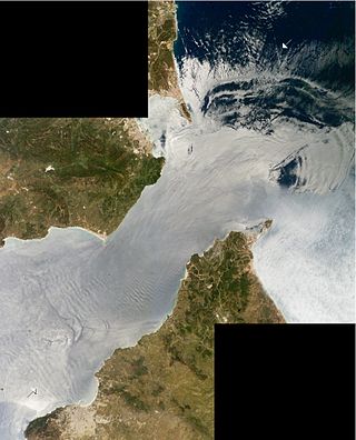
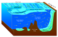
Internal waves are gravity waves that oscillate within a fluid medium, rather than on its surface. To exist, the fluid must be stratified: the density must change with depth/height due to changes, for example, in temperature and/or salinity. If the density changes over a small vertical distance, the waves propagate horizontally like surface waves, but do so at slower speeds as determined by the density difference of the fluid below and above the interface. If the density changes continuously, the waves can propagate vertically as well as horizontally through the fluid.

In fluid dynamics, dispersion of water waves generally refers to frequency dispersion, which means that waves of different wavelengths travel at different phase speeds. Water waves, in this context, are waves propagating on the water surface, with gravity and surface tension as the restoring forces. As a result, water with a free surface is generally considered to be a dispersive medium.

<span class="mw-page-title-main">Stokes flow</span> Type of fluid flow

Stokes flow, also named creeping flow or creeping motion, is a type of fluid flow where advective inertial forces are small compared with viscous forces. The Reynolds number is low, i.e. . This is a typical situation in flows where the fluid velocities are very slow, the viscosities are very large, or the length-scales of the flow are very small. Creeping flow was first studied to understand lubrication. In nature, this type of flow occurs in the swimming of microorganisms and sperm. In technology, it occurs in paint, MEMS devices, and in the flow of viscous polymers generally.

In physics, the acoustic wave equation is a second-order partial differential equation that governs the propagation of acoustic waves through a material medium resp. a standing wavefield. The equation describes the evolution of acoustic pressure p or particle velocity u as a function of position x and time t. A simplified (scalar) form of the equation describes acoustic waves in only one spatial dimension, while a more general form describes waves in three dimensions. Propagating waves in a pre-defined direction can also be calculated using a first order one-way wave equation.

In fluid mechanics, potential vorticity (PV) is a quantity which is proportional to the dot product of vorticity and stratification. This quantity, following a parcel of air or water, can only be changed by diabatic or frictional processes. It is a useful concept for understanding the generation of vorticity in cyclogenesis, especially along the polar front, and in analyzing flow in the ocean.

<span class="mw-page-title-main">Shallow water equations</span> Set of partial differential equations that describe the flow below a pressure surface in a fluid

The shallow-water equations (SWE) are a set of hyperbolic partial differential equations that describe the flow below a pressure surface in a fluid. The shallow-water equations in unidirectional form are also called Saint-Venant equations, after Adhémar Jean Claude Barré de Saint-Venant.

The derivation of the Navier–Stokes equations as well as their application and formulation for different families of fluids, is an important exercise in fluid dynamics with applications in mechanical engineering, physics, chemistry, heat transfer, and electrical engineering. A proof explaining the properties and bounds of the equations, such as Navier–Stokes existence and smoothness, is one of the important unsolved problems in mathematics.

<span class="mw-page-title-main">Stokes drift</span> Average velocity of a fluid parcel in a gravity wave

For a pure wave motion in fluid dynamics, the Stokes drift velocity is the average velocity when following a specific fluid parcel as it travels with the fluid flow. For instance, a particle floating at the free surface of water waves, experiences a net Stokes drift velocity in the direction of wave propagation.

<span class="mw-page-title-main">Stokes wave</span> Nonlinear and periodic surface wave on an inviscid fluid layer of constant mean depth

In fluid dynamics, a Stokes wave is a nonlinear and periodic surface wave on an inviscid fluid layer of constant mean depth. This type of modelling has its origins in the mid 19th century when Sir George Stokes – using a perturbation series approach, now known as the Stokes expansion – obtained approximate solutions for nonlinear wave motion.

<span class="mw-page-title-main">Mild-slope equation</span> Physics phenomenon and formula

In fluid dynamics, the mild-slope equation describes the combined effects of diffraction and refraction for water waves propagating over bathymetry and due to lateral boundaries—like breakwaters and coastlines. It is an approximate model, deriving its name from being originally developed for wave propagation over mild slopes of the sea floor. The mild-slope equation is often used in coastal engineering to compute the wave-field changes near harbours and coasts.

<span class="mw-page-title-main">Radiation stress</span> Term in physical oceanography

In fluid dynamics, the radiation stress is the depth-integrated – and thereafter phase-averaged – excess momentum flux caused by the presence of the surface gravity waves, which is exerted on the mean flow. The radiation stresses behave as a second-order tensor.

In physical oceanography and fluid mechanics, the Miles-Phillips mechanism describes the generation of wind waves from a flat sea surface by two distinct mechanisms. Wind blowing over the surface generates tiny wavelets. These wavelets develop over time and become ocean surface waves by absorbing the energy transferred from the wind. The Miles-Phillips mechanism is a physical interpretation of these wind-generated surface waves.
Both mechanisms are applied to gravity-capillary waves and have in common that waves are generated by a resonance phenomenon. The Miles mechanism is based on the hypothesis that waves arise as an instability of the sea-atmosphere system. The Phillips mechanism assumes that turbulent eddies in the atmospheric boundary layer induce pressure fluctuations at the sea surface. The Phillips mechanism is generally assumed to be important in the first stages of wave growth, whereas the Miles mechanism is important in later stages where the wave growth becomes exponential in time.

Nonlinear tides are generated by hydrodynamic distortions of tides. A tidal wave is said to be nonlinear when its shape deviates from a pure sinusoidal wave. In mathematical terms, the wave owes its nonlinearity due to the nonlinear advection and frictional terms in the governing equations. These become more important in shallow-water regions such as in estuaries. Nonlinear tides are studied in the fields of coastal morphodynamics, coastal engineering and physical oceanography. The nonlinearity of tides has important implications for the transport of sediment.

References

Historical

Further reading