Adiabatic invariant

Last updated

A property of a physical system, such as the entropy of a gas, that stays approximately constant when changes occur slowly is called an adiabatic invariant. By this it is meant that if a system is varied between two end points, as the time for the variation between the end points is increased to infinity, the variation of an adiabatic invariant between the two end points goes to zero.

Contents

In thermodynamics, an adiabatic process is a change that occurs without heat flow; it may be slow or fast. A reversible adiabatic process is an adiabatic process that occurs slowly compared to the time to reach equilibrium. In a reversible adiabatic process, the system is in equilibrium at all stages and the entropy is constant. In the 1st half of the 20th century the scientists that worked in quantum physics used the term "adiabatic" for reversible adiabatic processes and later for any gradually changing conditions which allow the system to adapt its configuration. The quantum mechanical definition is closer to the thermodynamical concept of a quasistatic process and has no direct relation with adiabatic processes in thermodynamics.

In mechanics, an adiabatic change is a slow deformation of the Hamiltonian, where the fractional rate of change of the energy is much slower than the orbital frequency. The area enclosed by the different motions in phase space are the adiabatic invariants.

In quantum mechanics, an adiabatic change is one that occurs at a rate much slower than the difference in frequency between energy eigenstates. In this case, the energy states of the system do not make transitions, so that the quantum number is an adiabatic invariant.

The old quantum theory was formulated by equating the quantum number of a system with its classical adiabatic invariant. This determined the form of the Bohr–Sommerfeld quantization rule: the quantum number is the area in phase space of the classical orbit.

Thermodynamics

In thermodynamics, adiabatic changes are those that do not increase the entropy. They occur slowly in comparison to the other characteristic timescales of the system of interest [1] and allow heat flow only between objects at the same temperature. For isolated systems, an adiabatic change allows no heat to flow in or out.

Adiabatic expansion of an ideal gas

If a container with an ideal gas is expanded instantaneously, the temperature of the gas doesn't change at all, because none of the molecules slow down. The molecules keep their kinetic energy, but now the gas occupies a bigger volume. If the container expands slowly, however, so that the ideal gas pressure law holds at any time, gas molecules lose energy at the rate that they do work on the expanding wall. The amount of work they do is the pressure times the area of the wall times the outward displacement, which is the pressure times the change in the volume of the gas:

If no heat enters the gas, the energy in the gas molecules is decreasing by the same amount. By definition, a gas is ideal when its temperature is only a function of the internal energy per particle, not the volume. So

where is the specific heat at constant volume. When the change in energy is entirely due to work done on the wall, the change in temperature is given by

This gives a differential relationship between the changes in temperature and volume, which can be integrated to find the invariant. The constant is just a unit conversion factor, which can be set equal to one:

So

is an adiabatic invariant, which is related to the entropy

Thus entropy is an adiabatic invariant. The N log(N) term makes the entropy additive, so the entropy of two volumes of gas is the sum of the entropies of each one.

In a molecular interpretation, S is the logarithm of the phase-space volume of all gas states with energy E(T) and volume V.

For a monatomic ideal gas, this can easily be seen by writing down the energy:

The different internal motions of the gas with total energy E define a sphere, the surface of a 3N-dimensional ball with radius . The volume of the sphere is

where is the gamma function.

Since each gas molecule can be anywhere within the volume V, the volume in phase space occupied by the gas states with energy E is

Since the N gas molecules are indistinguishable, the phase-space volume is divided by , the number of permutations of N molecules.

Using Stirling's approximation for the gamma function, and ignoring factors that disappear in the logarithm after taking N large,

Since the specific heat of a monatomic gas is 3/2, this is the same as the thermodynamic formula for the entropy.

Wien's law – adiabatic expansion of a box of light

For a box of radiation, ignoring quantum mechanics, the energy of a classical field in thermal equilibrium is infinite, since equipartition demands that each field mode has an equal energy on average, and there are infinitely many modes. This is physically ridiculous, since it means that all energy leaks into high-frequency electromagnetic waves over time.

Still, without quantum mechanics, there are some things that can be said about the equilibrium distribution from thermodynamics alone, because there is still a notion of adiabatic invariance that relates boxes of different size.

When a box is slowly expanded, the frequency of the light recoiling from the wall can be computed from the Doppler shift. If the wall is not moving, the light recoils at the same frequency. If the wall is moving slowly, the recoil frequency is only equal in the frame where the wall is stationary. In the frame where the wall is moving away from the light, the light coming in is bluer than the light coming out by twice the Doppler shift factor v/c:

On the other hand, the energy in the light is also decreased when the wall is moving away, because the light is doing work on the wall by radiation pressure. Because the light is reflected, the pressure is equal to twice the momentum carried by light, which is E/c. The rate at which the pressure does work on the wall is found by multiplying by the velocity:

This means that the change in frequency of the light is equal to the work done on the wall by the radiation pressure. The light that is reflected is changed both in frequency and in energy by the same amount:

Since moving the wall slowly should keep a thermal distribution fixed, the probability that the light has energy E at frequency f must only be a function of E/f.

This function cannot be determined from thermodynamic reasoning alone, and Wien guessed at the form that was valid at high frequency. He supposed that the average energy in high-frequency modes was suppressed by a Boltzmann-like factor:

This is not the expected classical energy in the mode, which is by equipartition, but a new and unjustified assumption that fit the high-frequency data.

When the expectation value is added over all modes in a cavity, this is Wien's distribution, and it describes the thermodynamic distribution of energy in a classical gas of photons. Wien's law implicitly assumes that light is statistically composed of packets that change energy and frequency in the same way. The entropy of a Wien gas scales as the volume to the power N, where N is the number of packets. This led Einstein to suggest that light is composed of localizable particles with energy proportional to the frequency. Then the entropy of the Wien gas can be given a statistical interpretation as the number of possible positions that the photons can be in.

Classical mechanics – action variables

Pendulum with extra small vibration, where
o
(
t
)
=
g
/
L
(
t
)
[?]
g
/
L
0
,
{\displaystyle \omega (t)={\sqrt {g/L(t)}}\approx {\sqrt {g/L_{0}}},}
and
L
(
t
)
[?]
L
0
+
e
(
t
)
.
{\displaystyle L(t)\approx L_{0}+\varepsilon (t).} Adiabatic-pendulum.png
Pendulum with extra small vibration, where and

Suppose that a Hamiltonian is slowly time-varying, for example, a one-dimensional harmonic oscillator with a changing frequency:

The action J of a classical orbit is the area enclosed by the orbit in phase space:

Since J is an integral over a full period, it is only a function of the energy. When the Hamiltonian is constant in time, and J is constant in time, the canonically conjugate variable increases in time at a steady rate:

So the constant can be used to change time derivatives along the orbit to partial derivatives with respect to at constant J. Differentiating the integral for J with respect to J gives an identity that fixes :

The integrand is the Poisson bracket of x and p. The Poisson bracket of two canonically conjugate quantities, like x and p, is equal to 1 in any canonical coordinate system. So

and is the inverse period. The variable increases by an equal amount in each period for all values of J  it is an angle variable.

Adiabatic invariance of J

The Hamiltonian is a function of J only, and in the simple case of the harmonic oscillator,

When H has no time dependence, J is constant. When H is slowly time-varying, the rate of change of J can be computed by re-expressing the integral for J:

The time derivative of this quantity is

Replacing time derivatives with theta derivatives, using and setting without loss of generality ( being a global multiplicative constant in the resulting time derivative of the action) yields

So as long as the coordinates J, do not change appreciably over one period, this expression can be integrated by parts to give zero. This means that for slow variations, there is no lowest-order change in the area enclosed by the orbit. This is the adiabatic invariance theorem  the action variables are adiabatic invariants.

For a harmonic oscillator, the area in phase space of an orbit at energy E is the area of the ellipse of constant energy,

The x radius of this ellipse is while the p radius of the ellipse is . Multiplying, the area is . So if a pendulum is slowly drawn in, such that the frequency changes, the energy changes by a proportional amount.

Old quantum theory

After Planck identified that Wien's law can be extended to all frequencies, even very low ones, by interpolating with the classical equipartition law for radiation, physicists wanted to understand the quantum behavior of other systems.

The Planck radiation law quantized the motion of the field oscillators in units of energy proportional to the frequency:

The quantum can only depend on the energy/frequency by adiabatic invariance, and since the energy must be additive when putting boxes end-to-end, the levels must be equally spaced.

Einstein, followed by Debye, extended the domain of quantum mechanics by considering the sound modes in a solid as quantized oscillators. This model explained why the specific heat of solids approached zero at low temperatures, instead of staying fixed at as predicted by classical equipartition.

At the Solvay conference, the question of quantizing other motions was raised, and Lorentz pointed out a problem, known as Rayleigh–Lorentz pendulum. If you consider a quantum pendulum whose string is shortened very slowly, the quantum number of the pendulum cannot change because at no point is there a high enough frequency to cause a transition between the states. But the frequency of the pendulum changes when the string is shorter, so the quantum states change energy.

Einstein responded that for slow pulling, the frequency and energy of the pendulum both change, but the ratio stays fixed. This is analogous to Wien's observation that under slow motion of the wall the energy to frequency ratio of reflected waves is constant. The conclusion was that the quantities to quantize must be adiabatic invariants.

This line of argument was extended by Sommerfeld into a general theory: the quantum number of an arbitrary mechanical system is given by the adiabatic action variable. Since the action variable in the harmonic oscillator is an integer, the general condition is

This condition was the foundation of the old quantum theory, which was able to predict the qualitative behavior of atomic systems. The theory is inexact for small quantum numbers, since it mixes classical and quantum concepts. But it was a useful half-way step to the new quantum theory.

Plasma physics

In plasma physics there are three adiabatic invariants of charged-particle motion.

The first adiabatic invariant, μ

The magnetic moment of a gyrating particle is

which respects special relativity. [2] is the relativistic Lorentz factor, is the rest mass, is the velocity perpendicular to the magnetic field, and is the magnitude of the magnetic field.

is a constant of the motion to all orders in an expansion in , where is the rate of any changes experienced by the particle, e.g., due to collisions or due to temporal or spatial variations in the magnetic field. Consequently, the magnetic moment remains nearly constant even for changes at rates approaching the gyrofrequency. When is constant, the perpendicular particle energy is proportional to , so the particles can be heated by increasing , but this is a "one-shot" deal because the field cannot be increased indefinitely. It finds applications in magnetic mirrors and magnetic bottles.

There are some important situations in which the magnetic moment is not invariant:

Magnetic pumping
If the collision frequency is larger than the pump frequency, μ is no longer conserved. In particular, collisions allow net heating by transferring some of the perpendicular energy to parallel energy.
Cyclotron heating
If B is oscillated at the cyclotron frequency, the condition for adiabatic invariance is violated, and heating is possible. In particular, the induced electric field rotates in phase with some of the particles and continuously accelerates them.
Magnetic cusps
The magnetic field at the center of a cusp vanishes, so the cyclotron frequency is automatically smaller than the rate of any changes. Thus the magnetic moment is not conserved, and particles are scattered relatively easily into the loss cone.

The second adiabatic invariant, J

The longitudinal invariant of a particle trapped in a magnetic mirror,

where the integral is between the two turning points, is also an adiabatic invariant. This guarantees, for example, that a particle in the magnetosphere moving around the Earth always returns to the same line of force. The adiabatic condition is violated in transit-time magnetic pumping, where the length of a magnetic mirror is oscillated at the bounce frequency, resulting in net heating.

The third adiabatic invariant, Φ

The total magnetic flux enclosed by a drift surface is the third adiabatic invariant, associated with the periodic motion of mirror-trapped particles drifting around the axis of the system. Because this drift motion is relatively slow, is often not conserved in practical applications.

Related Research Articles

<span class="mw-page-title-main">Angular momentum</span> Conserved physical quantity; rotational analogue of linear momentum

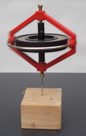
In physics, angular momentum is the rotational analog of linear momentum. It is an important physical quantity because it is a conserved quantity – the total angular momentum of a closed system remains constant. Angular momentum has both a direction and a magnitude, and both are conserved. Bicycles and motorcycles, flying discs, rifled bullets, and gyroscopes owe their useful properties to conservation of angular momentum. Conservation of angular momentum is also why hurricanes form spirals and neutron stars have high rotational rates. In general, conservation limits the possible motion of a system, but it does not uniquely determine it.

<span class="mw-page-title-main">Equations of motion</span> Equations that describe the behavior of a physical system

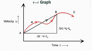
In physics, equations of motion are equations that describe the behavior of a physical system in terms of its motion as a function of time. More specifically, the equations of motion describe the behavior of a physical system as a set of mathematical functions in terms of dynamic variables. These variables are usually spatial coordinates and time, but may include momentum components. The most general choice are generalized coordinates which can be any convenient variables characteristic of the physical system. The functions are defined in a Euclidean space in classical mechanics, but are replaced by curved spaces in relativity. If the dynamics of a system is known, the equations are the solutions for the differential equations describing the motion of the dynamics.

<span class="mw-page-title-main">Four-vector</span> 4-dimensional vector in relativity

In special relativity, a four-vector is an object with four components, which transform in a specific way under Lorentz transformations. Specifically, a four-vector is an element of a four-dimensional vector space considered as a representation space of the standard representation of the Lorentz group, the representation. It differs from a Euclidean vector in how its magnitude is determined. The transformations that preserve this magnitude are the Lorentz transformations, which include spatial rotations and boosts.

A prior probability distribution of an uncertain quantity, often simply called the prior, is its assumed probability distribution before some evidence is taken into account. For example, the prior could be the probability distribution representing the relative proportions of voters who will vote for a particular politician in a future election. The unknown quantity may be a parameter of the model or a latent variable rather than an observable variable.

In information geometry, the Fisher information metric is a particular Riemannian metric which can be defined on a smooth statistical manifold, i.e., a smooth manifold whose points are probability measures defined on a common probability space. It can be used to calculate the informational difference between measurements.

In mathematical statistics, the Fisher information is a way of measuring the amount of information that an observable random variable X carries about an unknown parameter θ of a distribution that models X. Formally, it is the variance of the score, or the expected value of the observed information.

In particle and condensed matter physics, Goldstone bosons or Nambu–Goldstone bosons (NGBs) are bosons that appear necessarily in models exhibiting spontaneous breakdown of continuous symmetries. They were discovered by Yoichiro Nambu in particle physics within the context of the BCS superconductivity mechanism, and subsequently elucidated by Jeffrey Goldstone, and systematically generalized in the context of quantum field theory. In condensed matter physics such bosons are quasiparticles and are known as Anderson–Bogoliubov modes.

In physics and astronomy, the Reissner–Nordström metric is a static solution to the Einstein–Maxwell field equations, which corresponds to the gravitational field of a charged, non-rotating, spherically symmetric body of mass M. The analogous solution for a charged, rotating body is given by the Kerr–Newman metric.

The adiabatic theorem is a concept in quantum mechanics. Its original form, due to Max Born and Vladimir Fock (1928), was stated as follows:

In theoretical physics, supersymmetric quantum mechanics is an area of research where supersymmetry are applied to the simpler setting of plain quantum mechanics, rather than quantum field theory. Supersymmetric quantum mechanics has found applications outside of high-energy physics, such as providing new methods to solve quantum mechanical problems, providing useful extensions to the WKB approximation, and statistical mechanics.

The old quantum theory is a collection of results from the years 1900–1925 which predate modern quantum mechanics. The theory was never complete or self-consistent, but was instead a set of heuristic corrections to classical mechanics. The theory has come to be understood as the semi-classical approximation to modern quantum mechanics. The main and final accomplishments of the old quantum theory were the determination of the modern form of the periodic table by Edmund Stoner and the Pauli exclusion principle which were both premised on the Arnold Sommerfeld enhancements to the Bohr model of the atom.

The Kuramoto model, first proposed by Yoshiki Kuramoto, is a mathematical model used in describing synchronization. More specifically, it is a model for the behavior of a large set of coupled oscillators. Its formulation was motivated by the behavior of systems of chemical and biological oscillators, and it has found widespread applications in areas such as neuroscience and oscillating flame dynamics. Kuramoto was quite surprised when the behavior of some physical systems, namely coupled arrays of Josephson junctions, followed his model.

<span class="mw-page-title-main">Fundamental thermodynamic relation</span>

In thermodynamics, the fundamental thermodynamic relation are four fundamental equations which demonstrate how four important thermodynamic quantities depend on variables that can be controlled and measured experimentally. Thus, they are essentially equations of state, and using the fundamental equations, experimental data can be used to determine sought-after quantities like G or H (enthalpy). The relation is generally expressed as a microscopic change in internal energy in terms of microscopic changes in entropy, and volume for a closed system in thermal equilibrium in the following way.

In fluid mechanics, potential vorticity (PV) is a quantity which is proportional to the dot product of vorticity and stratification. This quantity, following a parcel of air or water, can only be changed by diabatic or frictional processes. It is a useful concept for understanding the generation of vorticity in cyclogenesis, especially along the polar front, and in analyzing flow in the ocean.

In classical mechanics, the Hannay angle is a mechanics analogue of the whirling geometric phase. It was named after John Hannay of the University of Bristol, UK. Hannay first described the angle in 1985, extending the ideas of the recently formalized Berry phase to classical mechanics.

The theoretical and experimental justification for the Schrödinger equation motivates the discovery of the Schrödinger equation, the equation that describes the dynamics of nonrelativistic particles. The motivation uses photons, which are relativistic particles with dynamics described by Maxwell's equations, as an analogue for all types of particles.

In physics, Berry connection and Berry curvature are related concepts which can be viewed, respectively, as a local gauge potential and gauge field associated with the Berry phase or geometric phase. The concept was first introduced by S. Pancharatnam as geometric phase and later elaborately explained and popularized by Michael Berry in a paper published in 1984 emphasizing how geometric phases provide a powerful unifying concept in several branches of classical and quantum physics.

In quantum information theory, the Wehrl entropy, named after Alfred Wehrl, is a classical entropy of a quantum-mechanical density matrix. It is a type of quasi-entropy defined for the Husimi Q representation of the phase-space quasiprobability distribution. See for a comprehensive review of basic properties of classical, quantum and Wehrl entropies, and their implications in statistical mechanics.

<span class="mw-page-title-main">Averaged Lagrangian</span>

In continuum mechanics, Whitham's averaged Lagrangian method – or in short Whitham's method – is used to study the Lagrangian dynamics of slowly-varying wave trains in an inhomogeneous (moving) medium. The method is applicable to both linear and non-linear systems. As a direct consequence of the averaging used in the method, wave action is a conserved property of the wave motion. In contrast, the wave energy is not necessarily conserved, due to the exchange of energy with the mean motion. However the total energy, the sum of the energies in the wave motion and the mean motion, will be conserved for a time-invariant Lagrangian. Further, the averaged Lagrangian has a strong relation to the dispersion relation of the system.

Rayleigh–Lorentz pendulum is a simple pendulum, but subjected to a slowly varying frequency due to an external action, named after Lord Rayleigh and Hendrik Lorentz. This problem formed the basis for the concept of adiabatic invariants in mechanics. On account of the slow variation of frequency, it is shown that the ratio of average energy to frequency is constant.

References

  1. Anosov, D. V.; Favorskii, A. P. (1988). "Adiabatic invariant". In Hazewinkel, Michiel (ed.). Encyclopedia of Mathematics. Vol. 1 (A-B). Reidel, Dordrecht. pp. 43–44. ISBN   9789401512398.
  2. Longair, Malcolm S. (2011). High Energy Astrophysics (3rd ed.). Cambridge: Cambridge University Press. p. 182. ISBN   978-0-521-75618-1.