Artificial neuron

Artificial neuron structure

An artificial neuron is a mathematical function conceived as a model of a biological neuron in a neural network. The artificial neuron is the elementary unit of an artificial neural network . ^[1]

The design of the artificial neuron was inspired by biological neural circuitry. Its inputs are analogous to excitatory postsynaptic potentials and inhibitory postsynaptic potentials at neural dendrites, or activation. Its weights are analogous to synaptic weights, and its output is analogous to a neuron's action potential which is transmitted along its axon.

Usually, each input is separately weighted, and the sum is often added to a term known as a bias (loosely corresponding to the threshold potential), before being passed through a nonlinear function known as an activation function. Depending on the task, these functions could have a sigmoid shape (e.g. for binary classification), but they may also take the form of other nonlinear functions, piecewise linear functions, or step functions. They are also often monotonically increasing, continuous, differentiable, and bounded. Non-monotonic, unbounded, and oscillating activation functions with multiple zeros that outperform sigmoidal and ReLU-like activation functions on many tasks have also been recently explored. The threshold function has inspired building logic gates referred to as threshold logic; applicable to building logic circuits resembling brain processing. For example, new devices such as memristors have been extensively used to develop such logic. ^[2]

The artificial neuron activation function should not be confused with a linear system's transfer function.

An artificial neuron may be referred to as a semi-linear unit, Nv neuron, binary neuron, linear threshold function, or McCulloch–Pitts (MCP) neuron, depending on the structure used.

Simple artificial neurons, such as the McCulloch–Pitts model, are sometimes described as "caricature models", since they are intended to reflect one or more neurophysiological observations, but without regard to realism. ^[3] Artificial neurons can also refer to artificial cells in neuromorphic engineering that are similar to natural physical neurons.

Basic structure

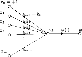
For a given artificial neuron ${\displaystyle k}$, let there be ${\displaystyle m+1}$ inputs with signals ${\displaystyle x_{0}}$ through ${\displaystyle x_{m}}$ and weights ${\displaystyle w_{k0}}$ through ${\displaystyle w_{km}}$. Usually, the input ${\displaystyle x_{0}}$ is assigned the value +1, which makes it a bias input with ${\displaystyle w_{k0}=b_{k}}$. This leaves only ${\displaystyle m}$ actual inputs to the neuron: ${\displaystyle x_{1}}$ to ${\displaystyle x_{m}}$.

The output of the ${\displaystyle k}$-th neuron is:

${\displaystyle y_{k}=\varphi \left(\sum _{j=0}^{m}w_{kj}x_{j}\right)}$,

where ${\displaystyle \varphi }$ (phi) is the activation function.

The output is analogous to the axon of a biological neuron, and its value propagates to the input of the next layer, through a synapse. It may also exit the system, possibly as part of an output vector.

It has no learning process as such. Its activation function weights are calculated, and its threshold value is predetermined.

McCulloch–Pitts (MCP) neuron

Main article: Perceptron

An MCP neuron is a kind of restricted artificial neuron which operates in discrete time-steps. Each has zero or more inputs, and are written as ${\displaystyle x_{1},...,x_{n}}$. It has one output, written as ${\displaystyle y}$. Each input can be either excitatory or inhibitory. The output can either be quiet or firing. An MCP neuron also has a threshold ${\displaystyle b\in \{0,1,2,...\}}$.

In an MCP neural network, all the neurons operate in synchronous discrete time-steps of ${\displaystyle t=0,1,2,3,...}$. At time ${\displaystyle t+1}$, the output of the neuron is ${\displaystyle y(t+1)=1}$ if the number of firing excitatory inputs is at least equal to the threshold, and no inhibitory inputs are firing; ${\displaystyle y(t+1)=0}$ otherwise.

Each output can be the input to an arbitrary number of neurons, including itself (i.e., self-loops are possible). However, an output cannot connect more than once with a single neuron. Self-loops do not cause contradictions, since the network operates in synchronous discrete time-steps.

As a simple example, consider a single neuron with threshold 0, and a single inhibitory self-loop. Its output would oscillate between 0 and 1 at every step, acting as a "clock".

Any finite state machine can be simulated by a MCP neural network. ^[4] Furnished with an infinite tape, MCP neural networks can simulate any Turing machine. ^[5]

Biological models

Main article: Biological neuron model

Neuron and myelinated axon, with signal flow from inputs at dendrites to outputs at axon terminals

Artificial neurons are designed to mimic aspects of their biological counterparts. However a significant performance gap exists between biological and artificial neural networks. In particular single biological neurons in the human brain with oscillating activation function capable of learning the XOR function have been discovered. ^[6]

• Dendrites – in biological neurons, dendrites act as the input vector. These dendrites allow the cell to receive signals from a large (>1000) number of neighboring neurons. As in the above mathematical treatment, each dendrite is able to perform "multiplication" by that dendrite's "weight value." The multiplication is accomplished by increasing or decreasing the ratio of synaptic neurotransmitters to signal chemicals introduced into the dendrite in response to the synaptic neurotransmitter. A negative multiplication effect can be achieved by transmitting signal inhibitors (i.e. oppositely charged ions) along the dendrite in response to the reception of synaptic neurotransmitters.
• Soma – in biological neurons, the soma acts as the summation function, seen in the above mathematical description. As positive and negative signals (exciting and inhibiting, respectively) arrive in the soma from the dendrites, the positive and negative ions are effectively added in summation, by simple virtue of being mixed together in the solution inside the cell's body.
• Axon – the axon gets its signal from the summation behavior which occurs inside the soma. The opening to the axon essentially samples the electrical potential of the solution inside the soma. Once the soma reaches a certain potential, the axon will transmit an all-in signal pulse down its length. In this regard, the axon behaves as the ability for us to connect our artificial neuron to other artificial neurons.

Unlike most artificial neurons, however, biological neurons fire in discrete pulses. Each time the electrical potential inside the soma reaches a certain threshold, a pulse is transmitted down the axon. This pulsing can be translated into continuous values. The rate (activations per second, etc.) at which an axon fires converts directly into the rate at which neighboring cells get signal ions introduced into them. The faster a biological neuron fires, the faster nearby neurons accumulate electrical potential (or lose electrical potential, depending on the "weighting" of the dendrite that connects to the neuron that fired). It is this conversion that allows computer scientists and mathematicians to simulate biological neural networks using artificial neurons which can output distinct values (often from −1 to 1).

Encoding

Research has shown that unary coding is used in the neural circuits responsible for birdsong production. ^{[7] [8]} The use of unary in biological networks is presumably due to the inherent simplicity of the coding. Another contributing factor could be that unary coding provides a certain degree of error correction. ^[9]

Physical artificial cells

There is research and development into physical artificial neurons – organic and inorganic.

For example, some artificial neurons can receive ^{[10] [11]} and release dopamine (chemical signals rather than electrical signals) and communicate with natural rat muscle and brain cells, with potential for use in BCIs/prosthetics. ^{[12] [13]}

Low-power biocompatible memristors may enable construction of artificial neurons which function at voltages of biological action potentials and could be used to directly process biosensing signals, for neuromorphic computing and/or direct communication with biological neurons. ^{[14] [15] [16]}

Organic neuromorphic circuits made out of polymers, coated with an ion-rich gel to enable a material to carry an electric charge like real neurons, have been built into a robot, enabling it to learn sensorimotorically within the real world, rather than via simulations or virtually. ^{[17] [18]} Moreover, artificial spiking neurons made of soft matter (polymers) can operate in biologically relevant environments and enable the synergetic communication between the artificial and biological domains. ^{[19] [20]}

History

The first artificial neuron was the Threshold Logic Unit (TLU), or Linear Threshold Unit, ^[21] first proposed by Warren McCulloch and Walter Pitts in 1943 in A logical calculus of the ideas immanent in nervous activity . The model was specifically targeted as a computational model of the "nerve net" in the brain. ^[22] As an activation function, it employed a threshold, equivalent to using the Heaviside step function. Initially, only a simple model was considered, with binary inputs and outputs, some restrictions on the possible weights, and a more flexible threshold value. Since the beginning it was already noticed that any Boolean function could be implemented by networks of such devices, what is easily seen from the fact that one can implement the AND and OR functions, and use them in the disjunctive or the conjunctive normal form. Researchers also soon realized that cyclic networks, with feedbacks through neurons, could define dynamical systems with memory, but most of the research concentrated (and still does) on strictly feed-forward networks because of the smaller difficulty they present.

One important and pioneering artificial neural network that used the linear threshold function was the perceptron, developed by Frank Rosenblatt. This model already considered more flexible weight values in the neurons, and was used in machines with adaptive capabilities. The representation of the threshold values as a bias term was introduced by Bernard Widrow in 1960 – see ADALINE.

In the late 1980s, when research on neural networks regained strength, neurons with more continuous shapes started to be considered. The possibility of differentiating the activation function allows the direct use of the gradient descent and other optimization algorithms for the adjustment of the weights. Neural networks also started to be used as a general function approximation model. The best known training algorithm called backpropagation has been rediscovered several times but its first development goes back to the work of Paul Werbos. ^{[23] [24]}

Types of activation function

Main article: Activation function

The activation function of a neuron is chosen to have a number of properties which either enhance or simplify the network containing the neuron. Crucially, for instance, any multilayer perceptron using a linear activation function has an equivalent single-layer network; a non-linear function is therefore necessary to gain the advantages of a multi-layer network.^{[ citation needed ]}

Below, ${\displaystyle u}$ refers in all cases to the weighted sum of all the inputs to the neuron, i.e. for ${\displaystyle n}$ inputs,

${\displaystyle u=\sum _{i=1}^{n}w_{i}x_{i}}$

where ${\displaystyle w}$ is a vector of synaptic weights and ${\displaystyle x}$ is a vector of inputs.

Step function

Main article: Step function

The output ${\displaystyle y}$ of this activation function is binary, depending on whether the input meets a specified threshold, ${\displaystyle \theta }$ (theta). The "signal" is sent, i.e. the output is set to 1, if the activation meets or exceeds the threshold.

${\displaystyle y={\begin{cases}1&{\text{if }}u\geq \theta \\0&{\text{if }}u<\theta \end{cases}}}$

This function is used in perceptrons, and appears in many other models. It performs a division of the space of inputs by a hyperplane. It is specially useful in the last layer of a network, intended for example to perform binary classification of the inputs.

Linear combination

Main article: Linear combination

In this case, the output unit is simply the weighted sum of its inputs, plus a bias term. A number of such linear neurons perform a linear transformation of the input vector. This is usually more useful in the early layers of a network. A number of analysis tools exist based on linear models, such as harmonic analysis, and they can all be used in neural networks with this linear neuron. The bias term allows us to make affine transformations to the data.

Sigmoid

Main article: Sigmoid function

A fairly simple nonlinear function, the sigmoid function such as the logistic function also has an easily calculated derivative, which can be important when calculating the weight updates in the network. It thus makes the network more easily manipulable mathematically, and was attractive to early computer scientists who needed to minimize the computational load of their simulations. It was previously commonly seen in multilayer perceptrons. However, recent work has shown sigmoid neurons to be less effective than rectified linear neurons. The reason is that the gradients computed by the backpropagation algorithm tend to diminish towards zero as activations propagate through layers of sigmoidal neurons, making it difficult to optimize neural networks using multiple layers of sigmoidal neurons.

Rectifier

Main article: Rectifier (neural networks)

In the context of artificial neural networks, the rectifier or ReLU (Rectified Linear Unit) is an activation function defined as the positive part of its argument:

${\displaystyle f(x)=x^{+}=\max(0,x),}$

where ${\displaystyle x}$ is the input to a neuron. This is also known as a ramp function and is analogous to half-wave rectification in electrical engineering. This activation function was first introduced to a dynamical network by Hahnloser et al. in a 2000 paper in Nature ^[25] with strong biological motivations and mathematical justifications. ^[26] It has been demonstrated for the first time in 2011 to enable better training of deeper networks, ^[27] compared to the widely used activation functions prior to 2011, i.e., the logistic sigmoid (which is inspired by probability theory; see logistic regression) and its more practical ^[28] counterpart, the hyperbolic tangent.

A commonly used variant of the ReLU activation function is the Leaky ReLU which allows a small, positive gradient when the unit is not active:

${\displaystyle f(x)={\begin{cases}x&{\text{if }}x>0,\\ax&{\text{otherwise}}.\end{cases}}}$

where ${\displaystyle x}$ is the input to the neuron and ${\displaystyle a}$ is a small positive constant (set to 0.01 in the original paper). ^[29]

Pseudocode algorithm

The following is a simple pseudocode implementation^{[ citation needed ]} of a single Threshold Logic Unit (TLU) which takes Boolean inputs (true or false), and returns a single Boolean output when activated. An object-oriented model is used. No method of training is defined, since several exist. If a purely functional model were used, the class TLU below would be replaced with a function TLU with input parameters threshold, weights, and inputs that returned a Boolean value.

class TLU defined as:data member threshold : number     data member weights : list of numbers of size X      function member fire(inputs : list of booleans of size X) : boolean defined as:variable T : number         T ← 0         for each i in 1 to X doif inputs(i) is true then                 T ← T + weights(i)             end ifend for eachif T > threshold thenreturn true         else:return false         end ifend functionend class

See also

• Binding neuron
• Connectionism

References

1. Rami A. Alzahrani; Alice C. Parker. "Neuromorphic Circuits With Neural Modulation Enhancing the Information Content of Neural Signaling". Proceedings of International Conference on Neuromorphic Systems 2020. Art. 19. New York: Association for Computing Machinery. doi: 10.1145/3407197.3407204 . ISBN   978-1-4503-8851-1. S2CID   220794387.
2. Maan, A. K.; Jayadevi, D. A.; James, A. P. (1 January 2016). "A Survey of Memristive Threshold Logic Circuits". IEEE Transactions on Neural Networks and Learning Systems. PP (99): 1734–1746. arXiv: 1604.07121 . Bibcode:2016arXiv160407121M. doi:10.1109/TNNLS.2016.2547842. ISSN   2162-237X. PMID   27164608. S2CID   1798273.
3. F. C. Hoppensteadt and E. M. Izhikevich (1997). Weakly connected neural networks. Springer. p. 4. ISBN   978-0-387-94948-2.
4. Minsky, Marvin Lee (1967-01-01). Computation: Finite and Infinite Machines. Prentice Hall. ISBN   978-0-13-165563-8.
5. McCulloch, Warren S.; Pitts, Walter (1943-12-01). "A logical calculus of the ideas immanent in nervous activity". The Bulletin of Mathematical Biophysics. 5 (4): 115–133. doi:10.1007/BF02478259. ISSN   1522-9602.
6. Gidon, Albert; Zolnik, Timothy Adam; Fidzinski, Pawel; Bolduan, Felix; Papoutsi, Athanasia; Poirazi, Panayiota; Holtkamp, Martin; Vida, Imre; Larkum, Matthew Evan (2020-01-03). "Dendritic action potentials and computation in human layer 2/3 cortical neurons". Science. 367 (6473): 83–87. Bibcode:2020Sci...367...83G. doi: 10.1126/science.aax6239 . PMID   31896716. S2CID   209676937.
7. Squire, L.; Albright, T.; Bloom, F.; Gage, F.; Spitzer, N., eds. (October 2007). Neural network models of birdsong production, learning, and coding (PDF). New Encyclopedia of Neuroscience: Elservier. Archived from the original (PDF) on 2015-04-12. Retrieved 12 April 2015.
8. Moore, J.M.; et al. (2011). "Motor pathway convergence predicts syllable repertoire size in oscine birds". Proc. Natl. Acad. Sci. USA. 108 (39): 16440–16445. Bibcode:2011PNAS..10816440M. doi: 10.1073/pnas.1102077108 . PMC   3182746 . PMID   21918109.
9. Potluri, Pushpa Sree (26 November 2014). "Error Correction Capacity of Unary Coding". arXiv: 1411.7406 [cs.IT].
10. Kleiner, Kurt (25 August 2022). "Making computer chips act more like brain cells". Knowable Magazine. doi:10.1146/knowable-082422-1 . Retrieved 23 September 2022.
11. Keene, Scott T.; Lubrano, Claudia; Kazemzadeh, Setareh; Melianas, Armantas; Tuchman, Yaakov; Polino, Giuseppina; Scognamiglio, Paola; Cinà, Lucio; Salleo, Alberto; van de Burgt, Yoeri; Santoro, Francesca (September 2020). "A biohybrid synapse with neurotransmitter-mediated plasticity". Nature Materials. 19 (9): 969–973. Bibcode:2020NatMa..19..969K. doi:10.1038/s41563-020-0703-y. ISSN   1476-4660. PMID   32541935. S2CID   219691307.
    • University press release: "Researchers develop artificial synapse that works with living cells". Stanford University via medicalxpress.com. Retrieved 23 September 2022.
12. "Artificial neuron swaps dopamine with rat brain cells like a real one". New Scientist. Retrieved 16 September 2022.
13. Wang, Ting; Wang, Ming; Wang, Jianwu; Yang, Le; Ren, Xueyang; Song, Gang; Chen, Shisheng; Yuan, Yuehui; Liu, Ruiqing; Pan, Liang; Li, Zheng; Leow, Wan Ru; Luo, Yifei; Ji, Shaobo; Cui, Zequn; He, Ke; Zhang, Feilong; Lv, Fengting; Tian, Yuanyuan; Cai, Kaiyu; Yang, Bowen; Niu, Jingyi; Zou, Haochen; Liu, Songrui; Xu, Guoliang; Fan, Xing; Hu, Benhui; Loh, Xian Jun; Wang, Lianhui; Chen, Xiaodong (8 August 2022). "A chemically mediated artificial neuron" . Nature Electronics. 5 (9): 586–595. doi:10.1038/s41928-022-00803-0. hdl: 10356/163240 . ISSN   2520-1131. S2CID   251464760.
14. "Scientists create tiny devices that work like the human brain". The Independent. April 20, 2020. Archived from the original on April 24, 2020. Retrieved May 17, 2020.
15. "Researchers unveil electronics that mimic the human brain in efficient learning". phys.org. Archived from the original on May 28, 2020. Retrieved May 17, 2020.
16. Fu, Tianda; Liu, Xiaomeng; Gao, Hongyan; Ward, Joy E.; Liu, Xiaorong; Yin, Bing; Wang, Zhongrui; Zhuo, Ye; Walker, David J. F.; Joshua Yang, J.; Chen, Jianhan; Lovley, Derek R.; Yao, Jun (April 20, 2020). "Bioinspired bio-voltage memristors". Nature Communications. 11 (1): 1861. Bibcode:2020NatCo..11.1861F. doi: 10.1038/s41467-020-15759-y . PMC   7171104 . PMID   32313096.
17. Bolakhe, Saugat. "Lego Robot with an Organic 'Brain' Learns to Navigate a Maze". Scientific American. Retrieved 1 February 2022.
18. Krauhausen, Imke; Koutsouras, Dimitrios A.; Melianas, Armantas; Keene, Scott T.; Lieberth, Katharina; Ledanseur, Hadrien; Sheelamanthula, Rajendar; Giovannitti, Alexander; Torricelli, Fabrizio; Mcculloch, Iain; Blom, Paul W. M.; Salleo, Alberto; Burgt, Yoeri van de; Gkoupidenis, Paschalis (December 2021). "Organic neuromorphic electronics for sensorimotor integration and learning in robotics". Science Advances. 7 (50): eabl5068. Bibcode:2021SciA....7.5068K. doi:10.1126/sciadv.abl5068. hdl:10754/673986. PMC   8664264 . PMID   34890232. S2CID   245046482.
19. Sarkar, Tanmoy; Lieberth, Katharina; Pavlou, Aristea; Frank, Thomas; Mailaender, Volker; McCulloch, Iain; Blom, Paul W. M.; Torriccelli, Fabrizio; Gkoupidenis, Paschalis (7 November 2022). "An organic artificial spiking neuron for in situ neuromorphic sensing and biointerfacing". Nature Electronics. 5 (11): 774–783. doi: 10.1038/s41928-022-00859-y . hdl: 10754/686016 . ISSN   2520-1131. S2CID   253413801.
20. "Artificial neurons emulate biological counterparts to enable synergetic operation". Nature Electronics. 5 (11): 721–722. 10 November 2022. doi:10.1038/s41928-022-00862-3. ISSN   2520-1131. S2CID   253469402.
21. Martin Anthony (January 2001). Discrete Mathematics of Neural Networks: Selected Topics. SIAM. pp. 3–. ISBN   978-0-89871-480-7.
22. Charu C. Aggarwal (25 July 2014). Data Classification: Algorithms and Applications. CRC Press. pp. 209–. ISBN   978-1-4665-8674-1.
23. Paul Werbos, Beyond Regression: New Tools for Prediction and Analysis in the Behavioral Sciences. PhD thesis, Harvard University, 1974
24. Werbos, P.J. (1990). "Backpropagation through time: what it does and how to do it". Proceedings of the IEEE. 78 (10): 1550–1560. doi:10.1109/5.58337. ISSN   0018-9219. S2CID   18470994.
25. Hahnloser, Richard H. R.; Sarpeshkar, Rahul; Mahowald, Misha A.; Douglas, Rodney J.; Seung, H. Sebastian (2000). "Digital selection and analogue amplification coexist in a cortex-inspired silicon circuit". Nature. 405 (6789): 947–951. Bibcode:2000Natur.405..947H. doi:10.1038/35016072. ISSN   0028-0836. PMID   10879535. S2CID   4399014.
26. R Hahnloser; H.S. Seung (2001). Permitted and Forbidden Sets in Symmetric Threshold-Linear Networks. NIPS 2001.
27. Xavier Glorot; Antoine Bordes; Yoshua Bengio (2011). Deep sparse rectifier neural networks (PDF). AISTATS.
28. Yann LeCun; Leon Bottou; Genevieve B. Orr; Klaus-Robert Müller (1998). "Efficient BackProp" (PDF). In G. Orr; K. Müller (eds.). Neural Networks: Tricks of the Trade. Springer.
29. Andrew L. Maas, Awni Y. Hannun, Andrew Y. Ng (2014). Rectifier Nonlinearities Improve Neural Network Acoustic Models.

Further reading

• McCulloch, Warren S.; Pitts, Walter (1943). "A logical calculus of the ideas immanent in nervous activity". Bulletin of Mathematical Biophysics. 5 (4): 115–133. doi:10.1007/bf02478259.
• Samardak, A.; Nogaret, A.; Janson, N. B.; Balanov, A. G.; Farrer, I.; Ritchie, D. A. (2009-06-05). "Noise-Controlled Signal Transmission in a Multithread Semiconductor Neuron". Physical Review Letters. 102 (22): 226802. Bibcode:2009PhRvL.102v6802S. doi:10.1103/physrevlett.102.226802. PMID   19658886. S2CID   11211062.

External links

• Artifical[sic] neuron mimicks function of human cells
• McCulloch-Pitts Neurons (Overview)