Dilution of precision (navigation)

Dilution of precision (DOP), or geometric dilution of precision (GDOP), is a term used in satellite navigation and geomatics engineering to specify the error propagation as a mathematical effect of navigation satellite geometry on positional measurement precision.

Understanding the geometric dilution of precision (GDOP) with a simple example. In A someone has measured the distance to two landmarks, and plotted their point as the intersection of two circles with the measured radius. In B the measurement has some error bounds, and their true location will lie anywhere in the green area. In C the measurement error is the same, but the error on their position has grown considerably due to the arrangement of the landmarks.

Navigation satellites with poor geometry for geometric dilution of precision (GDOP).

Navigation satellites with good geometry for geometric dilution of precision (GDOP).

Introduction

The concept of dilution of precision (DOP) originated with users of the Loran-C navigation system. ^[1] The idea of geometric DOP is to state how errors in the measurement will affect the final state estimation. This can be defined as: ^[2]

${\displaystyle \operatorname {GDOP} ={\frac {\Delta ({\text{output location}})}{\Delta ({\text{measured data}})}}}$

Conceptually you can geometrically imagine errors on a measurement resulting in the ${\displaystyle \Delta ({\text{measured data}})}$ term changing. Ideally small changes in the measured data will not result in large changes in output location. The opposite of this ideal is the situation where the solution is very sensitive to measurement errors. The interpretation of this formula is shown in the figure to the right, showing two possible scenarios with acceptable and poor GDOP.

More recently, the term has come into much wider usage with the development and adoption of GPS. Neglecting ionospheric ^[3] and tropospheric ^[4] effects, the signal from navigation satellites has a fixed precision. Therefore, the relative satellite-receiver geometry plays a major role in determining the precision of estimated positions and times. Due to the relative geometry of any given satellite to a receiver, the precision in the pseudorange of the satellite translates to a corresponding component in each of the four dimensions of position measured by the receiver (i.e., ${\displaystyle x}$, ${\displaystyle y}$, ${\displaystyle z}$, and ${\displaystyle t}$). The precision of multiple satellites in view of a receiver combine according to the relative position of the satellites to determine the level of precision in each dimension of the receiver measurement. When visible navigation satellites are close together in the sky, the geometry is said to be weak and the DOP value is high; when far apart, the geometry is strong and the DOP value is low. Consider two overlapping rings, or annuli, of different centres. If they overlap at right angles, the greatest extent of the overlap is much smaller than if they overlap in near parallel. Thus a low DOP value represents a better positional precision due to the wider angular separation between the satellites used to calculate a unit's position. Other factors that can increase the effective DOP are obstructions such as nearby mountains or buildings.

DOP can be expressed as a number of separate measurements:

HDOP

Horizontal dilution of precision

VDOP

Vertical dilution of precision

PDOP

Position (3D) dilution of precision

TDOP

Time dilution of precision

GDOP

Geometric dilution of precision

These values follow mathematically from the positions of the usable satellites. Signal receivers allow the display of these positions (skyplot) as well as the DOP values.

The term can also be applied to other location systems that employ several geographical spaced sites. It can occur in electronic-counter-counter-measures (electronic warfare) when computing the location of enemy emitters (radar jammers and radio communications devices). Using such an interferometry technique can provide certain geometric layout where there are degrees of freedom that cannot be accounted for due to inadequate configurations.

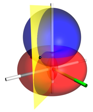
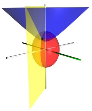
The effect of geometry of the satellites on position error is called geometric dilution of precision (GDOP) and it is roughly interpreted as ratio of position error to the range error. Imagine that a square pyramid is formed by lines joining four satellites with the receiver at the tip of the pyramid. The larger the volume of the pyramid, the better (lower) the value of GDOP; the smaller its volume, the worse (higher) the value of GDOP will be. Similarly, the greater the number of satellites, the better the value of GDOP.

Interpretation

DOP value	Rating [5]	Description
<1	Ideal	Highest possible confidence level to be used for applications demanding the highest possible precision at all times.
1–2	Excellent	At this confidence level, positional measurements are considered accurate enough to meet all but the most sensitive applications.
2–5	Good	Represents a level that marks the minimum appropriate for making accurate decisions. Positional measurements could be used to make reliable in-route navigation suggestions to the user.
5–10	Moderate	Positional measurements could be used for calculations, but the fix quality could still be improved. A more open view of the sky is recommended.
10–20	Fair	Represents a low confidence level. Positional measurements should be discarded or used only to indicate a very rough estimate of the current location.
>20	Poor	At this level, measurements should be discarded.

The DOP factors are functions of the diagonal elements of the covariance matrix of the parameters, expressed either in a global or a local geodetic frame.

Computation

As a first step in computing DOP, consider the unit vectors from the receiver to satellite i:

${\displaystyle {\begin{aligned}&\left({\frac {x_{i}-x}{R_{i}}},{\frac {y_{i}-y}{R_{i}}},{\frac {z_{i}-z}{R_{i}}}\right),&R_{i}&={\sqrt {(x_{i}-x)^{2}+(y_{i}-y)^{2}+(z_{i}-z)^{2}}}\end{aligned}}}$

where ${\displaystyle x,y,z}$ denote the position of the receiver and ${\displaystyle x_{i},y_{i},z_{i}}$ denote the position of satellite i. Formulate the matrix, A, which (for 4 pseudorange measurement residual equations) is:

${\displaystyle A={\begin{bmatrix}{\frac {x_{1}-x}{R_{1}}}&{\frac {y_{1}-y}{R_{1}}}&{\frac {z_{1}-z}{R_{1}}}&1\\{\frac {x_{2}-x}{R_{2}}}&{\frac {y_{2}-y}{R_{2}}}&{\frac {z_{2}-z}{R_{2}}}&1\\{\frac {x_{3}-x}{R_{3}}}&{\frac {y_{3}-y}{R_{3}}}&{\frac {z_{3}-z}{R_{3}}}&1\\{\frac {x_{4}-x}{R_{4}}}&{\frac {y_{4}-y}{R_{4}}}&{\frac {z_{4}-z}{R_{4}}}&1\end{bmatrix}}}$

The first three elements of each row of A are the components of a unit vector from the receiver to the indicated satellite. The last element of each row refers to the partial derivative of pseudorange w.r.t. receiver's clock bias. Formulate the matrix, Q, as the covariance matrix resulting from the least-squares normal matrix:

${\displaystyle Q=\left(A^{\mathsf {T}}A\right)^{-1}}$

In general:

${\displaystyle Q=\left(J_{\mathsf {x}}^{\mathsf {T}}\left(J_{d}C_{d}J_{d}^{\mathsf {T}}\right)^{-1}J_{x}\right)^{-1}}$

where ${\displaystyle J_{x}}$ is the Jacobian of the sensor measurement residual equations ${\displaystyle f_{i}\left({\underline {x}},{\underline {d}}\right)=0}$, with respect to the unknowns, ${\displaystyle {\underline {x}}}$; ${\displaystyle J_{d}}$ is the Jacobian of the sensor measurement residual equations with respect to the measured quantities ${\displaystyle {\underline {d}}}$, and ${\displaystyle C_{d}}$ is the correlation matrix for noise in the measured quantities.

For the preceding case of 4 range measurement residual equations: ${\displaystyle {\underline {x}}=(x,y,z,\tau )^{\mathsf {T}}}$, ${\displaystyle {\underline {d}}=\left(\tau _{1},\tau _{2},\tau _{3},\tau _{4}\right)^{\mathsf {T}}}$, ${\displaystyle \tau =ct}$, ${\displaystyle \tau _{i}=ct_{i}}$, ${\displaystyle R_{i}=|\tau _{i}-\tau |={\sqrt {(\tau _{i}-\tau )^{2}}}}$, ${\displaystyle f_{i}\left({\underline {x}},{\underline {d}}\right)={\sqrt {(x_{i}-x)^{2}+(y_{i}-y)^{2}+(z_{i}-z)^{2}}}-{\sqrt {(\tau _{i}-\tau )^{2}}}}$, ${\displaystyle J_{x}=A}$, ${\displaystyle J_{d}=-I}$ and the measurement noises for the different ${\displaystyle \tau _{i}}$ have been assumed to be independent which makes ${\displaystyle C_{d}=I}$.

This formula for Q arises from applying best linear unbiased estimation to a linearized version of the sensor measurement residual equations about the current solution ${\displaystyle \Delta {\underline {x}}=-Q*\left(J_{x}^{\mathsf {T}}\left(J_{d}C_{d}J_{d}^{\mathsf {T}}\right)^{-1}f\right)}$, except in the case of B.L.U.E. ${\displaystyle C_{d}}$ is a noise covariance matrix rather than the noise correlation matrix used in DOP, and the reason DOP makes this substitution is to obtain a relative error. When ${\displaystyle C_{d}}$ is a noise covariance matrix, ${\displaystyle Q}$ is an estimate of the matrix of covariance of noise in the unknowns due to the noise in the measured quantities. It is the estimate obtained by the first-order second moment (F.O.S.M.) uncertainty quantification technique which was state of the art in the 1980s. In order for the F.O.S.M. theory to be strictly applicable, either the input noise distributions need to be Gaussian or the measurement noise standard deviations need to be small relative to rate of change in the output near the solution. In this context, the second criteria is typically the one that is satisfied.

This (i.e. for the 4 time of arrival/range measurement residual equations) computation is in accordance with [6] where the weighting matrix, ${\displaystyle P=\left(J_{d}C_{d}J_{d}^{\mathsf {T}}\right)^{-1}}$ happens to simplify down to the identity matrix.

Note that P only simplifies down to the identity matrix because all the sensor measurement residual equations are time of arrival (pseudo range) equations. In other cases, for example when trying to locate someone broadcasting on an international distress frequency, ${\displaystyle P}$ would not simplify down to the identity matrix and in that case there would be a "frequency DOP" or FDOP component either in addition to or in place of the TDOP component. (Regarding "in place of the TDOP component": Since the clocks on the legacy International Cospas-Sarsat Programme LEO satellites are much less accurate than GPS clocks, discarding their time measurements would actually increase the geolocation solution accuracy.)

The elements of ${\displaystyle Q}$ are designated as:

${\displaystyle Q={\begin{bmatrix}\sigma _{x}^{2}&\sigma _{xy}&\sigma _{xz}&\sigma _{xt}\\\sigma _{xy}&\sigma _{y}^{2}&\sigma _{yz}&\sigma _{yt}\\\sigma _{xz}&\sigma _{yz}&\sigma _{z}^{2}&\sigma _{zt}\\\sigma _{xt}&\sigma _{yt}&\sigma _{zt}&\sigma _{t}^{2}\end{bmatrix}}}$

PDOP, TDOP, and GDOP are given by: ^[6]

${\displaystyle {\begin{aligned}\operatorname {PDOP} &={\sqrt {\sigma _{x}^{2}+\sigma _{y}^{2}+\sigma _{z}^{2}}}\\\operatorname {TDOP} &={\sqrt {\sigma _{t}^{2}}}\\\operatorname {GDOP} &={\sqrt {\operatorname {PDOP} ^{2}+\operatorname {TDOP} ^{2}}}\\\end{aligned}}}$

Notice GDOP is the square root of the trace of the ${\displaystyle Q}$ matrix.

The horizontal and vertical dilution of precision,

${\displaystyle {\begin{aligned}\operatorname {HDOP} &={\sqrt {\sigma _{n}^{2}+\sigma _{e}^{2}}}\\\operatorname {VDOP} &={\sqrt {\sigma _{u}^{2}}}\end{aligned}}}$,

are both dependent on the coordinate system used. To correspond to the local horizon plane and the local vertical in either a north, east, up coordinate system.

EDOP^2   x      x      x  x     NDOP^2   x      x  x       x    VDOP^2   x  x       x      x    TDOP^2

derived DOPs:

${\displaystyle {\begin{aligned}\operatorname {GDOP} &={\sqrt {\operatorname {EDOP} ^{2}+\operatorname {NDOP} ^{2}+\operatorname {VDOP} ^{2}+\operatorname {TDOP} ^{2}}}\\\operatorname {HDOP} &={\sqrt {\operatorname {EDOP} ^{2}+\operatorname {NDOP} ^{2}}}\\\operatorname {PDOP} &={\sqrt {\operatorname {EDOP} ^{2}+\operatorname {NDOP} ^{2}+\operatorname {VDOP} ^{2}}}\end{aligned}}}$

See also

• Circular error probable
• GNSS positioning calculation

References

1. Richard B. Langley (May 1999). "Dilution of Precision" (PDF). GPS World. Archived (PDF) from the original on 2011-10-04. Retrieved 2011-10-12.
2. Dudek, Gregory; Jenkin, Michael (2000). Computational Principles of Mobile Robotics . Cambridge University Press. ISBN   0-521-56876-5.
3. Paul Kintner, Cornell University; Todd Humphreys; University of Texas-Austin; Joanna Hinks; Cornell University (July–August 2009). "GNSS and Ionospheric Scintillation: How to Survive the Next Solar Maximum". Inside GNSS . Archived from the original on 2011-11-06. Retrieved 2011-10-12.
4. "GPS errors (Trimble tutorial)". Archived from the original on 2016-03-07. Retrieved 2016-02-08.
5. Isik, Oguz Kagan; Hong, Juhyeon; Petrunin, Ivan; Tsourdos, Antonios (25 August 2020). "Integrity Analysis for GPS-Based Navigation of UAVs in Urban Environment". Robotics. 9 (3): 66. doi: 10.3390/robotics9030066 .
6. Section 1.4.9 of Principles of Satellite Positioning.

Further reading

• DOP Factors
• manually calculating GDOP
• HDOP AND GPS HORIZONTAL POSITION ERRORS

• Article on DOP and Trimble's program: Determining Local GPS Satellite Geometry Effects On Position Accuracy.
• Notes & GIF image on manually calculating GDOP: Geographer's Craft
• GPS Errors & Estimating Your Receiver's Accuracy: Sam Wormley's GPS Accuracy Web Page
• GPS Accuracy, Errors & Precision: Radio-Electronics.com Archived 2014-02-22 at the Wayback Machine