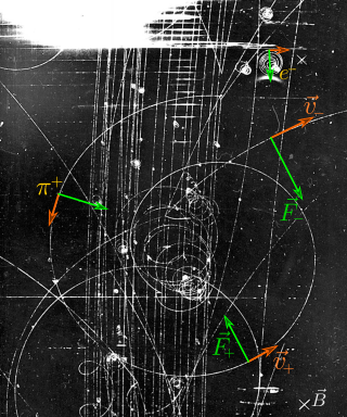
In physics, specifically in electromagnetism, the Lorentz force law is the combination of electric and magnetic force on a point charge due to electromagnetic fields. The Lorentz force, on the other hand, is a physical effect that occurs in the vicinity of electrically neutral, current-carrying conductors causing moving electrical charges to experience a magnetic force.

The Navier–Stokes equations are partial differential equations which describe the motion of viscous fluid substances. They were named after French engineer and physicist Claude-Louis Navier and the Irish physicist and mathematician George Gabriel Stokes. They were developed over several decades of progressively building the theories, from 1822 (Navier) to 1842–1850 (Stokes).

In probability theory and statistics, the multivariate normal distribution, multivariate Gaussian distribution, or joint normal distribution is a generalization of the one-dimensional (univariate) normal distribution to higher dimensions. One definition is that a random vector is said to be k-variate normally distributed if every linear combination of its k components has a univariate normal distribution. Its importance derives mainly from the multivariate central limit theorem. The multivariate normal distribution is often used to describe, at least approximately, any set of (possibly) correlated real-valued random variables, each of which clusters around a mean value.
In physics, a Langevin equation is a stochastic differential equation describing how a system evolves when subjected to a combination of deterministic and fluctuating ("random") forces. The dependent variables in a Langevin equation typically are collective (macroscopic) variables changing only slowly in comparison to the other (microscopic) variables of the system. The fast (microscopic) variables are responsible for the stochastic nature of the Langevin equation. One application is to Brownian motion, which models the fluctuating motion of a small particle in a fluid.

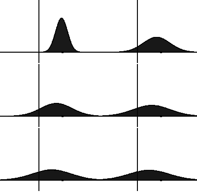
In statistical mechanics and information theory, the Fokker–Planck equation is a partial differential equation that describes the time evolution of the probability density function of the velocity of a particle under the influence of drag forces and random forces, as in Brownian motion. The equation can be generalized to other observables as well. The Fokker-Planck equation has multiple applications in information theory, graph theory, data science, finance, economics etc.

In statistics and control theory, Kalman filtering is an algorithm that uses a series of measurements observed over time, including statistical noise and other inaccuracies, to produce estimates of unknown variables that tend to be more accurate than those based on a single measurement, by estimating a joint probability distribution over the variables for each time-step. The filter is constructed as a mean squared error minimiser, but an alternative derivation of the filter is also provided showing how the filter relates to maximum likelihood statistics. The filter is named after Rudolf E. Kálmán.

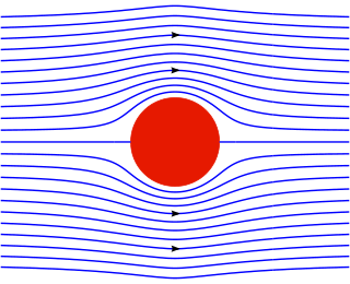
In fluid dynamics, two types of stream function are defined:
A stochastic differential equation (SDE) is a differential equation in which one or more of the terms is a stochastic process, resulting in a solution which is also a stochastic process. SDEs have many applications throughout pure mathematics and are used to model various behaviours of stochastic models such as stock prices, random growth models or physical systems that are subjected to thermal fluctuations.
In stochastic processes, the Stratonovich integral or Fisk–Stratonovich integral is a stochastic integral, the most common alternative to the Itô integral. Although the Itô integral is the usual choice in applied mathematics, the Stratonovich integral is frequently used in physics.

In geometry, a three-dimensional space is a mathematical space in which three values (coordinates) are required to determine the position of a point. Most commonly, it is the three-dimensional Euclidean space, that is, the Euclidean space of dimension three, which models physical space. More general three-dimensional spaces are called 3-manifolds. The term may also refer colloquially to a subset of space, a three-dimensional region, a solid figure.

In electromagnetism, charge density is the amount of electric charge per unit length, surface area, or volume. Volume charge density is the quantity of charge per unit volume, measured in the SI system in coulombs per cubic meter (C⋅m−3), at any point in a volume. Surface charge density (σ) is the quantity of charge per unit area, measured in coulombs per square meter (C⋅m−2), at any point on a surface charge distribution on a two dimensional surface. Linear charge density (λ) is the quantity of charge per unit length, measured in coulombs per meter (C⋅m−1), at any point on a line charge distribution. Charge density can be either positive or negative, since electric charge can be either positive or negative.
In control theory, the linear–quadratic–Gaussian (LQG) control problem is one of the most fundamental optimal control problems, and it can also be operated repeatedly for model predictive control. It concerns linear systems driven by additive white Gaussian noise. The problem is to determine an output feedback law that is optimal in the sense of minimizing the expected value of a quadratic cost criterion. Output measurements are assumed to be corrupted by Gaussian noise and the initial state, likewise, is assumed to be a Gaussian random vector.

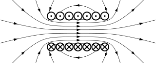
There are various mathematical descriptions of the electromagnetic field that are used in the study of electromagnetism, one of the four fundamental interactions of nature. In this article, several approaches are discussed, although the equations are in terms of electric and magnetic fields, potentials, and charges with currents, generally speaking.
The ensemble Kalman filter (EnKF) is a recursive filter suitable for problems with a large number of variables, such as discretizations of partial differential equations in geophysical models. The EnKF originated as a version of the Kalman filter for large problems, and it is now an important data assimilation component of ensemble forecasting. EnKF is related to the particle filter but the EnKF makes the assumption that all probability distributions involved are Gaussian; when it is applicable, it is much more efficient than the particle filter.
In mathematics – specifically, in stochastic analysis – an Itô diffusion is a solution to a specific type of stochastic differential equation. That equation is similar to the Langevin equation used in physics to describe the Brownian motion of a particle subjected to a potential in a viscous fluid. Itô diffusions are named after the Japanese mathematician Kiyosi Itô.
The Cauchy momentum equation is a vector partial differential equation put forth by Cauchy that describes the non-relativistic momentum transport in any continuum.
In filtering theory the Kushner equation is an equation for the conditional probability density of the state of a stochastic non-linear dynamical system, given noisy measurements of the state. It therefore provides the solution of the nonlinear filtering problem in estimation theory. The equation is sometimes referred to as the Stratonovich–Kushnerequation. However, the correct equation in terms of Itō calculus was first derived by Kushner although a more heuristic Stratonovich version of it appeared already in Stratonovich's works in late fifties. However, the derivation in terms of Itō calculus is due to Richard Bucy.
In stochastic analysis, a rough path is a generalization of the notion of smooth path allowing to construct a robust solution theory for controlled differential equations driven by classically irregular signals, for example a Wiener process. The theory was developed in the 1990s by Terry Lyons. Several accounts of the theory are available.
Quantum stochastic calculus is a generalization of stochastic calculus to noncommuting variables. The tools provided by quantum stochastic calculus are of great use for modeling the random evolution of systems undergoing measurement, as in quantum trajectories. Just as the Lindblad master equation provides a quantum generalization to the Fokker–Planck equation, quantum stochastic calculus allows for the derivation of quantum stochastic differential equations (QSDE) that are analogous to classical Langevin equations.
Projection filters are a set of algorithms based on stochastic analysis and information geometry, or the differential geometric approach to statistics, used to find approximate solutions for filtering problems for nonlinear state-space systems. The filtering problem consists of estimating the unobserved signal of a random dynamical system from partial noisy observations of the signal. The objective is computing the probability distribution of the signal conditional on the history of the noise-perturbed observations. This distribution allows for calculations of all statistics of the signal given the history of observations. If this distribution has a density, the density satisfies specific stochastic partial differential equations (SPDEs) called Kushner-Stratonovich equation, or Zakai equation. It is known that the nonlinear filter density evolves in an infinite dimensional function space.


