Inverted pendulum

Balancing cart, a simple robotics system circa 1976. The cart contains a servo system which monitors the angle of the rod and moves the cart back and forth to keep it upright.

An inverted pendulum is a pendulum that has its center of mass above its pivot point. It is unstable and without additional help will fall over. It can be suspended stably in this inverted position by using a control system to monitor the angle of the pole and move the pivot point horizontally back under the center of mass when it starts to fall over, keeping it balanced. The inverted pendulum is a classic problem in dynamics and control theory and is used as a benchmark for testing control strategies. It is often implemented with the pivot point mounted on a cart that can move horizontally under control of an electronic servo system as shown in the photo; this is called a cart and pole apparatus. ^[1] Most applications limit the pendulum to 1 degree of freedom by affixing the pole to an axis of rotation. Whereas a normal pendulum is stable when hanging downwards, an inverted pendulum is inherently unstable, and must be actively balanced in order to remain upright; this can be done either by applying a torque at the pivot point, by moving the pivot point horizontally as part of a feedback system, changing the rate of rotation of a mass mounted on the pendulum on an axis parallel to the pivot axis and thereby generating a net torque on the pendulum, or by oscillating the pivot point vertically. A simple demonstration of moving the pivot point in a feedback system is achieved by balancing an upturned broomstick on the end of one's finger.

A second type of inverted pendulum is a tiltmeter for tall structures, which consists of a wire anchored to the bottom of the foundation and attached to a float in a pool of oil at the top of the structure that has devices for measuring movement of the neutral position of the float away from its original position.

Overview

A pendulum with its bob hanging directly below the support pivot is at a stable equilibrium point; there is no torque on the pendulum so it will remain motionless, and if displaced from this position will experience a restoring torque which returns it toward the equilibrium position. A pendulum with its bob in an inverted position, supported on a rigid rod directly above the pivot, 180° from its stable equilibrium position, is at an unstable equilibrium point. At this point again there is no torque on the pendulum, but the slightest displacement away from this position will cause a gravitation torque on the pendulum which will accelerate it away from equilibrium, and it will fall over.

In order to stabilize a pendulum in this inverted position, a feedback control system can be used, which monitors the pendulum's angle and moves the position of the pivot point sideways when the pendulum starts to fall over, to keep it balanced. The inverted pendulum is a classic problem in dynamics and control theory and is widely used as a benchmark for testing control algorithms (PID controllers, state-space representation, neural networks, fuzzy control, genetic algorithms, etc.). Variations on this problem include multiple links, allowing the motion of the cart to be commanded while maintaining the pendulum, and balancing the cart-pendulum system on a see-saw. The inverted pendulum is related to rocket or missile guidance, where the center of gravity is located behind the center of drag causing aerodynamic instability. ^[2] The understanding of a similar problem can be shown by simple robotics in the form of a balancing cart. Balancing an upturned broomstick on the end of one's finger is a simple demonstration, and the problem is solved by self-balancing personal transporters such as the Segway PT, the self-balancing hoverboard and the self-balancing unicycle.

Another way that an inverted pendulum may be stabilized, without any feedback or control mechanism, is by oscillating the pivot rapidly up and down. This is called Kapitza's pendulum. If the oscillation is sufficiently strong (in terms of its acceleration and amplitude) then the inverted pendulum can recover from perturbations in a strikingly counterintuitive manner. If the driving point moves in simple harmonic motion, the pendulum's motion is described by the Mathieu equation. ^[3]

Equations of motion

The equations of motion of inverted pendulums are dependent on what constraints are placed on the motion of the pendulum. Inverted pendulums can be created in various configurations resulting in a number of Equations of Motion describing the behavior of the pendulum.

Stationary pivot point

In a configuration where the pivot point of the pendulum is fixed in space, the equation of motion is similar to that for an uninverted pendulum. The equation of motion below assumes no friction or any other resistance to movement, a rigid massless rod, and the restriction to 2-dimensional movement.

${\displaystyle {\ddot {\theta }}-{g \over \ell }\sin \theta =0}$

Where ${\displaystyle {\ddot {\theta }}}$ is the angular acceleration of the pendulum, ${\displaystyle g}$ is the standard gravity on the surface of the Earth, ${\displaystyle \ell }$ is the length of the pendulum, and ${\displaystyle \theta }$ is the angular displacement measured from the equilibrium position.

When ${\displaystyle {\ddot {\theta }}}$ added to both sides, it will have the same sign as the angular acceleration term:

${\displaystyle {\ddot {\theta }}={g \over \ell }\sin \theta }$

Thus, the inverted pendulum will accelerate away from the vertical unstable equilibrium in the direction initially displaced, and the acceleration is inversely proportional to the length. Tall pendulums fall more slowly than short ones.

Derivation using torque and moment of inertia:

A schematic drawing of the inverted pendulum on a cart. The rod is considered massless. The mass of the cart and the point mass at the end of the rod are denoted by M and m. The rod has a length l.

The pendulum is assumed to consist of a point mass, of mass ${\displaystyle m}$, affixed to the end of a massless rigid rod, of length ${\displaystyle \ell }$, attached to a pivot point at the end opposite the point mass.

The net torque of the system must equal the moment of inertia times the angular acceleration:

${\displaystyle {\boldsymbol {\tau }}_{\mathrm {net} }=I{\ddot {\theta }}}$

The torque due to gravity providing the net torque:

${\displaystyle {\boldsymbol {\tau }}_{\mathrm {net} }=mg\ell \sin \theta \,\!}$

Where ${\displaystyle \theta \ }$ is the angle measured from the inverted equilibrium position.

The resulting equation:

${\displaystyle I{\ddot {\theta }}=mg\ell \sin \theta \,\!}$

The moment of inertia for a point mass:

${\displaystyle I=mR^{2}}$

In the case of the inverted pendulum the radius is the length of the rod, ${\displaystyle \ell }$.

Substituting in ${\displaystyle I=m\ell ^{2}}$

${\displaystyle m\ell ^{2}{\ddot {\theta }}=mg\ell \sin \theta \,\!}$

Mass and ${\displaystyle \ell ^{2}}$ is divided from each side resulting in:

${\displaystyle {\ddot {\theta }}={g \over \ell }\sin \theta }$

Inverted pendulum on a cart

An inverted pendulum on a cart consists of a mass ${\displaystyle m}$ at the top of a pole of length ${\displaystyle \ell }$ pivoted on a horizontally moving base as shown in the adjacent image. The cart is restricted to linear motion and is subject to forces resulting in or hindering motion.

Essentials of stabilization

The essentials of stabilizing the inverted pendulum can be summarized qualitatively in three steps.

The simple stabilizing control system used on the cart with wine glass above.

1. If the tilt angle ${\displaystyle \theta }$ is to the right, the cart must accelerate to the right and vice versa.

2. The position of the cart ${\displaystyle x}$ relative to track center is stabilized by slightly modulating the null angle (the angle error that the control system tries to null) by the position of the cart, that is, null angle ${\displaystyle =\theta +kx}$ where ${\displaystyle k}$ is small. This makes the pole want to lean slightly toward track center and stabilize at track center where the tilt angle is exactly vertical. Any offset in the tilt sensor or track slope that would otherwise cause instability translates into a stable position offset. A further added offset gives position control.

3. A normal pendulum subject to a moving pivot point such as a load lifted by a crane, has a peaked response at the pendulum radian frequency of ${\displaystyle \omega _{p}={\sqrt {g/\ell }}}$. To prevent uncontrolled swinging, the frequency spectrum of the pivot motion should be suppressed near ${\displaystyle \omega _{p}}$. The inverted pendulum requires the same suppression filter to achieve stability.

Note that, as a consequence of the null angle modulation strategy, the position feedback is positive, that is, a sudden command to move right will produce an initial cart motion to the left followed by a move right to rebalance the pendulum. The interaction of the pendulum instability and the positive position feedback instability to produce a stable system is a feature that makes the mathematical analysis an interesting and challenging problem.

From Lagrange's equations

The equations of motion can be derived using Lagrange's equations. We refer to the drawing to the right where ${\displaystyle \theta (t)}$ is the angle of the pendulum of length ${\displaystyle l}$ with respect to the vertical direction and the acting forces are gravity and an external force F in the x-direction. Define ${\displaystyle x(t)}$ to be the position of the cart.

The kinetic energy ${\displaystyle T}$ of the system is:

${\displaystyle T={\frac {1}{2}}Mv_{1}^{2}+{\frac {1}{2}}mv_{2}^{2},}$

where ${\displaystyle v_{1}}$ is the velocity of the cart and ${\displaystyle v_{2}}$ is the velocity of the point mass ${\displaystyle m}$. ${\displaystyle v_{1}}$ and ${\displaystyle v_{2}}$ can be expressed in terms of x and ${\displaystyle \theta }$ by writing the velocity as the first derivative of the position;

${\displaystyle v_{1}^{2}={\dot {x}}^{2},}$

${\displaystyle v_{2}^{2}=\left({\frac {\rm {d}}{{\rm {d}}t}}{\left(x-\ell \sin \theta \right)}\right)^{2}+\left({\frac {\rm {d}}{{\rm {d}}t}}{\left(\ell \cos \theta \right)}\right)^{2}.}$

Simplifying the expression for ${\displaystyle v_{2}}$ leads to:

${\displaystyle v_{2}^{2}={\dot {x}}^{2}-2\ell {\dot {x}}{\dot {\theta }}\cos \theta +\ell ^{2}{\dot {\theta }}^{2}.}$

The kinetic energy is now given by:

${\displaystyle T={\frac {1}{2}}\left(M+m\right){\dot {x}}^{2}-m\ell {\dot {x}}{\dot {\theta }}\cos \theta +{\frac {1}{2}}m\ell ^{2}{\dot {\theta }}^{2}.}$

The generalized coordinates of the system are ${\displaystyle \theta }$ and ${\displaystyle x}$, each has a generalized force. On the ${\displaystyle x}$ axis, the generalized force ${\displaystyle Q_{x}}$ can be calculated through its virtual work

${\displaystyle Q_{x}\delta x=F\delta x,\quad Q_{x}=F,}$

on the ${\displaystyle \theta }$ axis, the generalized force ${\displaystyle Q_{\theta }}$ can be also calculated through its virtual work

${\displaystyle Q_{\theta }\delta \theta =mgl\sin \theta \delta \theta ,\quad Q_{\theta }=mgl\sin \theta .}$

According to the Lagrange's equations, the equations of motion are:

${\displaystyle {\frac {\mathrm {d} }{\mathrm {d} t}}{\partial {T} \over \partial {\dot {x}}}-{\partial {T} \over \partial x}=F,}$

${\displaystyle {\frac {\mathrm {d} }{\mathrm {d} t}}{\partial {T} \over \partial {\dot {\theta }}}-{\partial {T} \over \partial \theta }=mgl\sin \theta ,}$

substituting ${\displaystyle T}$ in these equations and simplifying leads to the equations that describe the motion of the inverted pendulum:

${\displaystyle \left(M+m\right){\ddot {x}}-m\ell {\ddot {\theta }}\cos \theta +m\ell {\dot {\theta }}^{2}\sin \theta =F,}$

${\displaystyle \ell {\ddot {\theta }}-g\sin \theta ={\ddot {x}}\cos \theta .}$

These equations are nonlinear, but since the goal of a control system would be to keep the pendulum upright the equations can be linearized around ${\displaystyle \theta \approx 0}$.

From Euler-Lagrange equations

The generalized forces can be both written as potential energy ${\displaystyle V_{x}}$ and ${\displaystyle V_{\theta }}$,

Generalized Forces	Potential Energy
${\displaystyle Q_{x}=F}$	${\displaystyle V_{x}=\int _{t_{0}}^{t}F{\dot {x}}\ {\rm {d}}t}$
${\displaystyle Q_{\theta }=mgl\sin \theta }$	${\displaystyle V_{\theta }=mgl\cos \theta }$

According to the D'Alembert's principle, generalized forces and potential energy are connected:

${\displaystyle Q_{j}={\frac {\mathrm {d} }{\mathrm {d} t}}{\frac {\partial V}{\partial {\dot {q}}_{j}}}-{\frac {\partial V}{\partial q_{j}}}\,,}$

However, under certain circumstances, the potential energy is not accessible, only generalized forces are available.

After getting the Lagrangian ${\displaystyle {\mathcal {L}}=T-V}$, we can also use Euler–Lagrange equation to solve for equations of motion:

${\displaystyle {\frac {\partial {\mathcal {L}}}{\partial x}}-{\frac {\mathrm {d} }{\mathrm {d} t}}\left({\frac {\partial {\mathcal {L}}}{\partial {\dot {x}}}}\right)=0}$,

${\displaystyle {\frac {\partial {\mathcal {L}}}{\partial \theta }}-{\frac {\mathrm {d} }{\mathrm {d} t}}\left({\frac {\partial {\mathcal {L}}}{\partial {\dot {\theta }}}}\right)=0}$.

The only difference is whether to incorporate the generalized forces into the potential energy ${\displaystyle V_{j}}$ or write them explicitly as ${\displaystyle Q_{j}}$ on the right side, they all lead to the same equations in the final.

From Newton's second law

Oftentimes it is beneficial to use Newton's second law instead of Lagrange's equations because Newton's equations give the reaction forces at the joint between the pendulum and the cart. These equations give rise to two equations for each body; one in the x-direction and the other in the y-direction. The equations of motion of the cart are shown below where the LHS is the sum of the forces on the body and the RHS is the acceleration.

${\displaystyle F-R_{x}=M{\ddot {x}}}$

${\displaystyle F_{N}-R_{y}-Mg=0}$

In the equations above ${\displaystyle R_{x}}$ and ${\displaystyle R_{y}}$ are reaction forces at the joint. ${\displaystyle F_{N}}$ is the normal force applied to the cart. This second equation only depends on the vertical reaction force thus the equation can be used to solve for the normal force. The first equation can be used to solve for the horizontal reaction force. In order to complete the equations of motion, the acceleration of the point mass attached to the pendulum must be computed. The position of the point mass can be given in inertial coordinates as

${\displaystyle {\vec {r}}_{P}=(x-\ell \sin \theta ){\hat {x}}_{I}+\ell \cos \theta {\hat {y}}_{I}}$

Taking two derivatives yields the acceleration vector in the inertial reference frame.

${\displaystyle {\vec {a}}_{P/I}=({\ddot {x}}+\ell {\dot {\theta }}^{2}\sin \theta -\ell {\ddot {\theta }}\cos \theta ){\hat {x}}_{I}+(-\ell {\dot {\theta }}^{2}\cos \theta -\ell {\ddot {\theta }}\sin \theta ){\hat {y}}_{I}}$

Then, using Newton's second law, two equations can be written in the x-direction and the y-direction. Note that the reaction forces are positive as applied to the pendulum and negative when applied to the cart. This is due to Newton's Third Law.

${\displaystyle R_{x}=m({\ddot {x}}+\ell {\dot {\theta }}^{2}\sin \theta -\ell {\ddot {\theta }}\cos \theta )}$

${\displaystyle R_{y}-mg=m(-\ell {\dot {\theta }}^{2}\cos \theta -\ell {\ddot {\theta }}\sin \theta )}$

The first equation allows yet another way to compute the horizontal reaction force in the event the applied force ${\displaystyle F}$ is not known. The second equation can be used to solve for the vertical reaction force. The first equation of motion is derived by substituting ${\displaystyle F-R_{x}=M{\ddot {x}}}$ into ${\displaystyle R_{x}=m({\ddot {x}}+\ell {\dot {\theta }}^{2}\sin \theta -\ell {\ddot {\theta }}\cos \theta )}$ which yields

${\displaystyle \left(M+m\right){\ddot {x}}-m\ell {\ddot {\theta }}\cos \theta +m\ell {\dot {\theta }}^{2}\sin \theta =F}$

By inspection this equation is identical to the result from Lagrange's Method. In order to obtain the second equation, the pendulum equation of motion must be dotted with a unit vector which runs perpendicular to the pendulum at all times and is typically noted as the x-coordinate of the body frame. In inertial coordinates this vector can be written using a simple 2-D coordinate transformation

${\displaystyle {\hat {x}}_{B}=\cos \theta {\hat {x}}_{I}+\sin \theta {\hat {y}}_{I}}$

The pendulum equation of motion written in vector form is ${\displaystyle \sum {\vec {F}}=m{\vec {a}}_{P/I}}$. Dotting ${\displaystyle {\hat {x}}_{B}}$ with both sides yields the following on the LHS (note that a transpose is the same as a dot product)

${\displaystyle ({\hat {x}}_{B})^{T}\sum {\vec {F}}=({\hat {x}}_{B})^{T}(R_{x}{\hat {x}}_{I}+R_{y}{\hat {y}}_{I}-mg{\hat {y}}_{I})=({\hat {x}}_{B})^{T}(R_{p}{\hat {y}}_{B}-mg{\hat {y}}_{I})=-mg\sin \theta }$

In the above equation the relationship between body frame components of the reaction forces and inertial frame components of reaction forces is used. The assumption that the bar connecting the point mass to the cart is massless implies that this bar cannot transfer any load perpendicular to the bar. Thus, the inertial frame components of the reaction forces can be written simply as ${\displaystyle R_{p}{\hat {y}}_{B}}$ which signifies that the bar can only transfer loads along the axis of the bar itself. This gives rise to another equation which can be used to solve for the tension in the rod itself

${\displaystyle R_{p}={\sqrt {R_{x}^{2}+R_{y}^{2}}}}$

The RHS of the equation is computed similarly by dotting ${\displaystyle {\hat {x}}_{B}}$ with the acceleration of the pendulum. The result (after some simplification) is shown below.

${\displaystyle m({\hat {x}}_{B})^{T}({\vec {a}}_{P/I})=m({\ddot {x}}\cos \theta -\ell {\ddot {\theta }})}$

Combining the LHS with the RHS and dividing through by m yields

${\displaystyle \ell {\ddot {\theta }}-g\sin \theta ={\ddot {x}}\cos \theta }$

which again is identical to the result of Lagrange's method. The benefit of using Newton's method is that all reaction forces are revealed to ensure that nothing will be damaged.

Variants

Achieving stability of an inverted pendulum has become a common engineering challenge for researchers. ^[4] There are different variations of the inverted pendulum on a cart ranging from a rod on a cart to a multiple segmented inverted pendulum on a cart. Another variation places the inverted pendulum's rod or segmented rod on the end of a rotating assembly. In both, (the cart and rotating system) the inverted pendulum can only fall in a plane. The inverted pendulums in these projects can either be required to only maintain balance after an equilibrium position is achieved or be able to achieve equilibrium by itself. Another platform is a two-wheeled balancing inverted pendulum. The two wheeled platform has the ability to spin on the spot offering a great deal of maneuverability. ^[5] Yet another variation balances on a single point. A spinning top, a unicycle, or an inverted pendulum atop a spherical ball all balance on a single point.

Drawing showing how a Kapitza pendulum can be constructed: a motor rotates a crank at a high speed, the crank vibrates a lever arm up and down, which the pendulum is attached to with a pivot.

Kapitza's pendulum

Main article: Kapitza's pendulum

An inverted pendulum in which the pivot is oscillated rapidly up and down can be stable in the inverted position. This is called Kapitza's pendulum, after Russian physicist Pyotr Kapitza who first analysed it. The equation of motion for a pendulum connected to a massless, oscillating base is derived the same way as with the pendulum on the cart. The position of the point mass is now given by:

${\displaystyle \left(-\ell \sin \theta ,y+\ell \cos \theta \right)}$

and the velocity is found by taking the first derivative of the position:

${\displaystyle v^{2}={\dot {y}}^{2}-2\ell {\dot {y}}{\dot {\theta }}\sin \theta +\ell ^{2}{\dot {\theta }}^{2}.}$

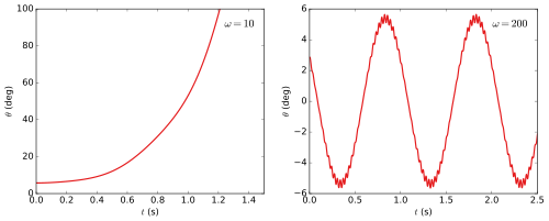
Plots for the inverted pendulum on an oscillatory base. The first plot shows the response of the pendulum on a slow oscillation, the second the response on a fast oscillation

The Lagrangian for this system can be written as:

${\displaystyle L={\frac {1}{2}}m\left({\dot {y}}^{2}-2\ell {\dot {y}}{\dot {\theta }}\sin \theta +\ell ^{2}{\dot {\theta }}^{2}\right)-mg\left(y+\ell \cos \theta \right)}$

and the equation of motion follows from:

${\displaystyle {\mathrm {d} \over \mathrm {d} t}{\partial {L} \over \partial {\dot {\theta }}}-{\partial {L} \over \partial \theta }=0}$

resulting in:

${\displaystyle \ell {\ddot {\theta }}-{\ddot {y}}\sin \theta =g\sin \theta .}$

If y represents a simple harmonic motion, ${\displaystyle y=A\sin \omega t}$, the following differential equation is:

${\displaystyle {\ddot {\theta }}-{g \over \ell }\sin \theta =-{A \over \ell }\omega ^{2}\sin \omega t\sin \theta .}$

This equation does not have elementary closed-form solutions, but can be explored in a variety of ways. It is closely approximated by the Mathieu equation, for instance, when the amplitude of oscillations are small. Analyses show that the pendulum stays upright for fast oscillations. The first plot shows that when ${\displaystyle y}$ is a slow oscillation, the pendulum quickly falls over when disturbed from the upright position. The angle ${\displaystyle \theta }$ exceeds 90° after a short time, which means the pendulum has fallen on the ground. If ${\displaystyle y}$ is a fast oscillation the pendulum can be kept stable around the vertical position. The second plot shows that when disturbed from the vertical position, the pendulum now starts an oscillation around the vertical position (${\displaystyle \theta =0}$). The deviation from the vertical position stays small, and the pendulum doesn't fall over.

Examples

Arguably the most prevalent example of a stabilized inverted pendulum is a human being. A person standing upright acts as an inverted pendulum with their feet as the pivot, and without constant small muscular adjustments would fall over. The human nervous system contains an unconscious feedback control system, the sense of balance or righting reflex, that uses proprioceptive input from the eyes, muscles and joints, and orientation input from the vestibular system consisting of the three semicircular canals in the inner ear, and two otolith organs, to make continual small adjustments to the skeletal muscles to keep us standing upright. Walking, running, or balancing on one leg puts additional demands on this system. Certain diseases and alcohol or drug intoxication can interfere with this reflex, causing dizziness and disequilibration, an inability to stand upright. A field sobriety test used by police to test drivers for the influence of alcohol or drugs, tests this reflex for impairment.

Some simple examples include balancing brooms or meter sticks by hand.

The inverted pendulum has been employed in various devices and trying to balance an inverted pendulum presents a unique engineering problem for researchers. ^[6] The inverted pendulum was a central component in the design of several early seismometers due to its inherent instability resulting in a measurable response to any disturbance. ^[7]

The inverted pendulum model has been used in some recent personal transporters, such as the two-wheeled self-balancing scooters and single-wheeled electric unicycles. These devices are kinematically unstable and use an electronic feedback servo system to keep them upright.

Swinging a pendulum on a cart into its inverted pendulum state is considered a traditional optimal control toy problem/benchmark. ^{[8] [9]}

Trajectory of a fixed time cartpole swing up that minimizes the force squared

See also

• Double inverted pendulum
• Inertia wheel pendulum
• Furuta pendulum
• iBOT
• Humanoid robot
• Ballbot

References

1. C.A. Hamilton Union College Senior Project 1966
2. "Model Rocket Stability".
3. Mitchell, Joe. "Techniques for the Oscillated Pendulum and the Mathieu Equation" (PDF). math.ou.edu. Retrieved 2023-11-06.
4. Ooi, Rich Chi. "Balancing a Two-Wheeled Autonomous Robot" (PDF). robotics.ee.uwa.edu.au. Retrieved 2023-11-06.
5. "Archived copy" (PDF). Archived from the original (PDF) on 2016-03-04. Retrieved 2012-05-01.
6. "Archived copy" (PDF). Archived from the original (PDF) on 2016-03-04. Retrieved 2012-05-01.
7. "The Early History of Seismometry (to 1900)". Archived from the original on 2009-11-28.
8. "The Acrobot and Cart-Pole" (PDF).
9. "Cart-Pole Swing-Up". www.cs.huji.ac.il. Retrieved 2019-08-19.

• D. Liberzon Switching in Systems and Control (2003 Springer) pp. 89ff

Further reading

• Franklin; et al. (2005). Feedback control of dynamic systems, 5, Prentice Hall. ISBN   0-13-149930-0

External links

• YouTube - Inverted Pendulum - Demo #3
• YouTube - inverted pendulum
• YouTube - Double Pendulum on a Cart
• YouTube - Triple Pendulum on a Cart
• A dynamical simulation of an inverse pendulum on an oscillatory base
• Inverted Pendulum: Analysis, Design, and Implementation
• Non-Linear Swing-Up and Stabilizing Control of an Inverted Pendulum System
• Stabilization fuzzy control of inverted pendulum systems ^{[ permanent dead link ]}
• Blog post on inverted pendulum, with Python code
• Equations of Motion for the Cart and Pole Control Task