It arose sequentially in two main published papers. The earlier version of the estimator was developed in 1956,[1] when Charles Stein reached a relatively shocking conclusion that while the then-usual estimate of the mean, the sample mean, is admissible when , it is inadmissible when . Stein proposed a possible improvement to the estimator that shrinks the sample means towards a more central mean vector (which can be chosen a priori or commonly as the "average of averages" of the sample means, given all samples share the same size). This observation is commonly referred to as Stein's example or paradox. In 1961, Willard James and Charles Stein simplified the original process.[2]
It can be shown that the James–Stein estimator dominates the "ordinary" least squares approach, meaning the James–Stein estimator has a lower or equal mean squared error than the "ordinary" least square estimator.
We are interested in obtaining an estimate, , of , based on a single observation, , of .
In real-world application, this is a common situation in which a set of parameters is sampled, and the samples are corrupted by independent Gaussian noise. Since this noise has mean of zero, it may be reasonable to use the samples themselves as an estimate of the parameters. This approach is the least squares estimator, which is .
Stein demonstrated that in terms of mean squared error, the least squares estimator, , is sub-optimal to shrinkage based estimators, such as the James–Stein estimator, .[1] The paradoxical result, that there is a (possibly) better and never any worse estimate of in mean squared error as compared to the sample mean, became known as Stein's example.
Formulation
MSE (R) of least squares estimator (ML) vs. James–Stein estimator (JS). The James–Stein estimator gives its best estimate when the norm of the actual parameter vector θ is near zero.
If is known, the James–Stein estimator is given by
James and Stein showed that the above estimator dominates for any , meaning that the James–Stein estimator always achieves lower mean squared error (MSE) than the maximum likelihood estimator.[2][4] By definition, this makes the least squares estimator inadmissible when .
Notice that if then this estimator simply takes the natural estimator and shrinks it towards the origin 0. In fact this is not the only direction of shrinkage that works. Let ν be an arbitrary fixed vector of dimension . Then there exists an estimator of the James–Stein type that shrinks toward ν, namely
The James–Stein estimator dominates the usual estimator for any ν. A natural question to ask is whether the improvement over the usual estimator is independent of the choice of ν. The answer is no. The improvement is small if is large. Thus to get a very great improvement some knowledge of the location of θ is necessary. Of course this is the quantity we are trying to estimate so we don't have this knowledge a priori. But we may have some guess as to what the mean vector is. This can be considered a disadvantage of the estimator: the choice is not objective as it may depend on the beliefs of the researcher. Nonetheless, James and Stein's result is that any finite guess ν improves the expected MSE over the maximum-likelihood estimator, which is tantamount to using an infinite ν, surely a poor guess.
Interpretation
Seeing the James–Stein estimator as an empirical Bayes method gives some intuition to this result: One assumes that θ itself is a random variable with prior distribution, where A is estimated from the data itself. Estimating A only gives an advantage compared to the maximum-likelihood estimator when the dimension is large enough; hence it does not work for . The James–Stein estimator is a member of a class of Bayesian estimators that dominate the maximum-likelihood estimator.[5]
A consequence of the above discussion is the following counterintuitive result: When three or more unrelated parameters are measured, their total MSE can be reduced by using a combined estimator such as the James–Stein estimator; whereas when each parameter is estimated separately, the least squares (LS) estimator is admissible. A quirky example would be estimating the speed of light, tea consumption in Taiwan, and hog weight in Montana, all together. The James–Stein estimator always improves upon the total MSE, i.e., the sum of the expected squared errors of each component. Therefore, the total MSE in measuring light speed, tea consumption, and hog weight would improve by using the James–Stein estimator. However, any particular component (such as the speed of light) would improve for some parameter values, and deteriorate for others. Thus, although the James–Stein estimator dominates the LS estimator when three or more parameters are estimated, any single component does not dominate the respective component of the LS estimator.
The conclusion from this hypothetical example is that measurements should be combined if one is interested in minimizing their total MSE. For example, in a telecommunication setting, it is reasonable to combine channel tap measurements in a channel estimation scenario, as the goal is to minimize the total channel estimation error.
The James–Stein estimator has also found use in fundamental quantum theory, where the estimator has been used to improve the theoretical bounds of the entropic uncertainty principle for more than three measurements.[6]
An intuitive derivation and interpretation is given by the Galtonian perspective.[7] Under this interpretation, we aim to predict the population means using the imperfectly measured sample means. The equation of the OLS estimator in a hypothetical regression of the population means on the sample means gives an estimator of the form of either the James–Stein estimator (when we force the OLS intercept to equal 0) or of the Efron-Morris estimator (when we allow the intercept to vary).
Improvements
Despite the intuition that the James–Stein estimator shrinks the maximum-likelihood estimate toward, the estimate actually moves away from for small values of as the multiplier on is then negative. This can be easily remedied by replacing this multiplier by zero when it is negative. The resulting estimator is called the positive-part James–Stein estimator and is given by
This estimator has a smaller risk than the basic James–Stein estimator. It follows that the basic James–Stein estimator is itself inadmissible.[8]
It turns out, however, that the positive-part estimator is also inadmissible.[4] This follows from a general result which requires admissible estimators to be smooth.
Extensions
The James–Stein estimator may seem at first sight to be a result of some peculiarity of the problem setting. In fact, the estimator exemplifies a very wide-ranging effect; namely, the fact that the "ordinary" or least squares estimator is often inadmissible for simultaneous estimation of several parameters.[citation needed] This effect has been called Stein's phenomenon, and has been demonstrated for several different problem settings, some of which are briefly outlined below.
James and Stein demonstrated that the estimator presented above can still be used when the variance is unknown, by replacing it with the standard estimator of the variance, . The dominance result still holds under the same condition, namely, .[2]
The results in this article are for the case when only a single observation vector y is available. For the more general case when vectors are available, the results are similar:
where is the -length average of the observations, and, therefore, .
The work of James and Stein has been extended to the case of a general measurement covariance matrix, i.e., where measurements may be statistically dependent and may have differing variances.[9] A similar dominating estimator can be constructed, with a suitably generalized dominance condition. This can be used to construct a linear regression technique which outperforms the standard application of the LS estimator.[9]
Stein's result has been extended to a wide class of distributions and loss functions. However, this theory provides only an existence result, in that explicit dominating estimators were not actually exhibited.[10] It is quite difficult to obtain explicit estimators improving upon the usual estimator without specific restrictions on the underlying distributions.[4]
In statistics, an estimator is a rule for calculating an estimate of a given quantity based on observed data: thus the rule, the quantity of interest and its result are distinguished. For example, the sample mean is a commonly used estimator of the population mean.
In statistics, maximum likelihood estimation (MLE) is a method of estimating the parameters of an assumed probability distribution, given some observed data. This is achieved by maximizing a likelihood function so that, under the assumed statistical model, the observed data is most probable. The point in the parameter space that maximizes the likelihood function is called the maximum likelihood estimate. The logic of maximum likelihood is both intuitive and flexible, and as such the method has become a dominant means of statistical inference.
In statistics, the mean squared error (MSE) or mean squared deviation (MSD) of an estimator measures the average of the squares of the errors—that is, the average squared difference between the estimated values and the actual value. MSE is a risk function, corresponding to the expected value of the squared error loss. The fact that MSE is almost always strictly positive is because of randomness or because the estimator does not account for information that could produce a more accurate estimate. In machine learning, specifically empirical risk minimization, MSE may refer to the empirical risk, as an estimate of the true MSE.
In probability and statistics, an exponential family is a parametric set of probability distributions of a certain form, specified below. This special form is chosen for mathematical convenience, including the enabling of the user to calculate expectations, covariances using differentiation based on some useful algebraic properties, as well as for generality, as exponential families are in a sense very natural sets of distributions to consider. The term exponential class is sometimes used in place of "exponential family", or the older term Koopman–Darmois family. Sometimes loosely referred to as "the" exponential family, this class of distributions is distinct because they all possess a variety of desirable properties, most importantly the existence of a sufficient statistic.
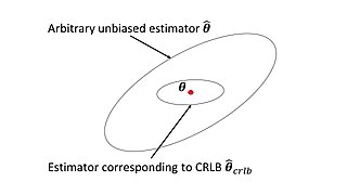
In estimation theory and statistics, the Cramér–Rao bound (CRB) relates to estimation of a deterministic parameter. The result is named in honor of Harald Cramér and Calyampudi Radhakrishna Rao, but has also been derived independently by Maurice Fréchet, Georges Darmois, and by Alexander Aitken and Harold Silverstone. It is also known as Fréchet-Cramér–Rao or Fréchet-Darmois-Cramér-Rao lower bound. It states that the precision of any unbiased estimator is at most the Fisher information; or (equivalently) the reciprocal of the Fisher information is a lower bound on its variance.
In statistics, the theory of minimum norm quadratic unbiased estimation (MINQUE) was developed by C. R. Rao. MINQUE is a theory alongside other estimation methods in estimation theory, such as the method of moments or maximum likelihood estimation. Similar to the theory of best linear unbiased estimation, MINQUE is specifically concerned with linear regression models. The method was originally conceived to estimate heteroscedastic error variance in multiple linear regression. MINQUE estimators also provide an alternative to maximum likelihood estimators or restricted maximum likelihood estimators for variance components in mixed effects models. MINQUE estimators are quadratic forms of the response variable and are used to estimate a linear function of the variances.
Estimation theory is a branch of statistics that deals with estimating the values of parameters based on measured empirical data that has a random component. The parameters describe an underlying physical setting in such a way that their value affects the distribution of the measured data. An estimator attempts to approximate the unknown parameters using the measurements. In estimation theory, two approaches are generally considered:
In statistics, ordinary least squares (OLS) is a type of linear least squares method for choosing the unknown parameters in a linear regression model by the principle of least squares: minimizing the sum of the squares of the differences between the observed dependent variable in the input dataset and the output of the (linear) function of the independent variable. Some sources consider OLS to be linear regression.
In probability theory, the Rice distribution or Rician distribution is the probability distribution of the magnitude of a circularly-symmetric bivariate normal random variable, possibly with non-zero mean (noncentral). It was named after Stephen O. Rice (1907–1986).
In decision theory and estimation theory, Stein's example is the observation that when three or more parameters are estimated simultaneously, there exist combined estimators more accurate on average than any method that handles the parameters separately. It is named after Charles Stein of Stanford University, who discovered the phenomenon in 1955.
In mathematics, the Ornstein–Uhlenbeck process is a stochastic process with applications in financial mathematics and the physical sciences. Its original application in physics was as a model for the velocity of a massive Brownian particle under the influence of friction. It is named after Leonard Ornstein and George Eugene Uhlenbeck.
In statistics, generalized least squares (GLS) is a method used to estimate the unknown parameters in a linear regression model. It is used when there is a non-zero amount of correlation between the residuals in the regression model. GLS is employed to improve statistical efficiency and reduce the risk of drawing erroneous inferences, as compared to conventional least squares and weighted least squares methods. It was first described by Alexander Aitken in 1935.
In estimation theory and decision theory, a Bayes estimator or a Bayes action is an estimator or decision rule that minimizes the posterior expected value of a loss function. Equivalently, it maximizes the posterior expectation of a utility function. An alternative way of formulating an estimator within Bayesian statistics is maximum a posteriori estimation.
In statistics, the multivariate t-distribution is a multivariate probability distribution. It is a generalization to random vectors of the Student's t-distribution, which is a distribution applicable to univariate random variables. While the case of a random matrix could be treated within this structure, the matrix t-distribution is distinct and makes particular use of the matrix structure.
In statistics, the bias of an estimator is the difference between this estimator's expected value and the true value of the parameter being estimated. An estimator or decision rule with zero bias is called unbiased. In statistics, "bias" is an objective property of an estimator. Bias is a distinct concept from consistency: consistent estimators converge in probability to the true value of the parameter, but may be biased or unbiased.
The topic of heteroskedasticity-consistent (HC) standard errors arises in statistics and econometrics in the context of linear regression and time series analysis. These are also known as heteroskedasticity-robust standard errors, Eicker–Huber–White standard errors, to recognize the contributions of Friedhelm Eicker, Peter J. Huber, and Halbert White.
In statistics, principal component regression (PCR) is a regression analysis technique that is based on principal component analysis (PCA). PCR is a form of reduced rank regression. More specifically, PCR is used for estimating the unknown regression coefficients in a standard linear regression model.
In statistics, efficiency is a measure of quality of an estimator, of an experimental design, or of a hypothesis testing procedure. Essentially, a more efficient estimator needs fewer input data or observations than a less efficient one to achieve the Cramér–Rao bound. An efficient estimator is characterized by having the smallest possible variance, indicating that there is a small deviance between the estimated value and the "true" value in the L2 norm sense.
Symmetries in quantum mechanics describe features of spacetime and particles which are unchanged under some transformation, in the context of quantum mechanics, relativistic quantum mechanics and quantum field theory, and with applications in the mathematical formulation of the standard model and condensed matter physics. In general, symmetry in physics, invariance, and conservation laws, are fundamentally important constraints for formulating physical theories and models. In practice, they are powerful methods for solving problems and predicting what can happen. While conservation laws do not always give the answer to the problem directly, they form the correct constraints and the first steps to solving a multitude of problems. In application, understanding symmetries can also provide insights on the eigenstates that can be expected. For example, the existence of degenerate states can be inferred by the presence of non commuting symmetry operators or that the non degenerate states are also eigenvectors of symmetry operators.
In statistics, the Innovation Method provides an estimator for the parameters of stochastic differential equations given a time series of observations of the state variables. In the framework of continuous-discrete state space models, the innovation estimator is obtained by maximizing the log-likelihood of the corresponding discrete-time innovation process with respect to the parameters. The innovation estimator can be classified as a M-estimator, a quasi-maximum likelihood estimator or a prediction error estimator depending on the inferential considerations that want to be emphasized. The innovation method is a system identification technique for developing mathematical models of dynamical systems from measured data and for the optimal design of experiments.
↑ Beran, R. (1995). THE ROLE OF HAJEK’S CONVOLUTION THEOREM IN STATISTICAL THEORY
1 2 3 Lehmann, E. L.; Casella, G. (1998), Theory of Point Estimation (2nded.), New York: Springer
↑ Efron, B.; Morris, C. (1973). "Stein's Estimation Rule and Its Competitors—An Empirical Bayes Approach". Journal of the American Statistical Association. 68 (341). American Statistical Association: 117–130. doi:10.2307/2284155. JSTOR2284155.
↑ Stander, M. (2017), Using Stein's estimator to correct the bound on the entropic uncertainty principle for more than two measurements, arXiv:1702.02440, Bibcode:2017arXiv170202440S
Judge, George G.; Bock, M. E. (1978). The Statistical Implications of Pre-Test and Stein-Rule Estimators in Econometrics. New York: North Holland. pp.229–257. ISBN0-7204-0729-X.
This page is based on this Wikipedia article Text is available under the CC BY-SA 4.0 license; additional terms may apply. Images, videos and audio are available under their respective licenses.