Related Research Articles

Distance is a numerical or occasionally qualitative measurement of how far apart objects, points, people, or ideas are. In physics or everyday usage, distance may refer to a physical length or an estimation based on other criteria. The term is also frequently used metaphorically to mean a measurement of the amount of difference between two similar objects or a degree of separation. Most such notions of distance, both physical and metaphorical, are formalized in mathematics using the notion of a metric space.
In probability theory, de Finetti's theorem states that exchangeable observations are conditionally independent relative to some latent variable. An epistemic probability distribution could then be assigned to this variable. It is named in honor of Bruno de Finetti.

In statistics, the Pearson correlation coefficient (PCC) is a correlation coefficient that measures linear correlation between two sets of data. It is the ratio between the covariance of two variables and the product of their standard deviations; thus, it is essentially a normalized measurement of the covariance, such that the result always has a value between −1 and 1. As with covariance itself, the measure can only reflect a linear correlation of variables, and ignores many other types of relationships or correlations. As a simple example, one would expect the age and height of a sample of children from a primary school to have a Pearson correlation coefficient significantly greater than 0, but less than 1.
The Ising model, named after the physicists Ernst Ising and Wilhelm Lenz, is a mathematical model of ferromagnetism in statistical mechanics. The model consists of discrete variables that represent magnetic dipole moments of atomic "spins" that can be in one of two states. The spins are arranged in a graph, usually a lattice, allowing each spin to interact with its neighbors. Neighboring spins that agree have a lower energy than those that disagree; the system tends to the lowest energy but heat disturbs this tendency, thus creating the possibility of different structural phases. The model allows the identification of phase transitions as a simplified model of reality. The two-dimensional square-lattice Ising model is one of the simplest statistical models to show a phase transition.
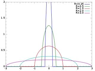
The Wigner semicircle distribution, named after the physicist Eugene Wigner, is the probability distribution defined on the domain [−R, R] whose probability density function f is a scaled semicircle, i.e. a semi-ellipse, centered at :
In probability theory and mathematical physics, a random matrix is a matrix-valued random variable—that is, a matrix in which some or all of its entries are sampled randomly from a probability distribution. Random matrix theory (RMT) is the study of properties of random matrices, often as they become large. RMT provides techniques like mean-field theory, diagrammatic methods, the cavity method, or the replica method to compute quantities like traces, spectral densities, or scalar products between eigenvectors. Many physical phenomena, such as the spectrum of nuclei of heavy atoms, the thermal conductivity of a lattice, or the emergence of quantum chaos, can be modeled mathematically as problems concerning large, random matrices.

The Wigner quasiprobability distribution is a quasiprobability distribution. It was introduced by Eugene Wigner in 1932 to study quantum corrections to classical statistical mechanics. The goal was to link the wavefunction that appears in Schrödinger's equation to a probability distribution in phase space.
Quantum tomography or quantum state tomography is the process by which a quantum state is reconstructed using measurements on an ensemble of identical quantum states. The source of these states may be any device or system which prepares quantum states either consistently into quantum pure states or otherwise into general mixed states. To be able to uniquely identify the state, the measurements must be tomographically complete. That is, the measured operators must form an operator basis on the Hilbert space of the system, providing all the information about the state. Such a set of observations is sometimes called a quorum. The term tomography was first used in the quantum physics literature in a 1993 paper introducing experimental optical homodyne tomography.
This glossary of statistics and probability is a list of definitions of terms and concepts used in the mathematical sciences of statistics and probability, their sub-disciplines, and related fields. For additional related terms, see Glossary of mathematics and Glossary of experimental design.
In quantum mechanics, the Wigner–Weyl transform or Weyl–Wigner transform is the invertible mapping between functions in the quantum phase space formulation and Hilbert space operators in the Schrödinger picture.
A quasiprobability distribution is a mathematical object similar to a probability distribution but which relaxes some of Kolmogorov's axioms of probability theory. Quasiprobability distributions arise naturally in the study of quantum mechanics when treated in phase space formulation, commonly used in quantum optics, time-frequency analysis, and elsewhere.

The Husimi Q representation, introduced by Kôdi Husimi in 1940, is a quasiprobability distribution commonly used in quantum mechanics to represent the phase space distribution of a quantum state such as light in the phase space formulation. It is used in the field of quantum optics and particularly for tomographic purposes. It is also applied in the study of quantum effects in superconductors.
In mathematics, the Fortuin–Kasteleyn–Ginibre (FKG) inequality is a correlation inequality, a fundamental tool in statistical mechanics and probabilistic combinatorics, due to Cees M. Fortuin, Pieter W. Kasteleyn, and Jean Ginibre. Informally, it says that in many random systems, increasing events are positively correlated, while an increasing and a decreasing event are negatively correlated. It was obtained by studying the random cluster model.

Gábor J. Székely is a Hungarian-American statistician/mathematician best known for introducing energy statistics (E-statistics). Examples include: the distance correlation, which is a bona fide dependence measure, equals zero exactly when the variables are independent; the distance skewness, which equals zero exactly when the probability distribution is diagonally symmetric; the E-statistic for normality test; and the E-statistic for clustering.
In quantum information theory, the Wehrl entropy, named after Alfred Wehrl, is a classical entropy of a quantum-mechanical density matrix. It is a type of quasi-entropy defined for the Husimi Q representation of the phase-space quasiprobability distribution. See for a comprehensive review of basic properties of classical, quantum and Wehrl entropies, and their implications in statistical mechanics.
The phase-space formulation is a formulation of quantum mechanics that places the position and momentum variables on equal footing in phase space. The two key features of the phase-space formulation are that the quantum state is described by a quasiprobability distribution and operator multiplication is replaced by a star product.

Robin Lyth Hudson was a British mathematician notable for his contribution to quantum probability.
In mathematics, the Segal–Bargmann space, also known as the Bargmann space or Bargmann–Fock space, is the space of holomorphic functions F in n complex variables satisfying the square-integrability condition:
First passage percolation is a mathematical method used to describe the paths reachable in a random medium within a given amount of time.
References
- ↑ Dirac, P. A. M. (1942). "Bakerian Lecture. The Physical Interpretation of Quantum Mechanics". Proceedings of the Royal Society A: Mathematical, Physical and Engineering Sciences. 180 (980): 1–39. Bibcode:1942RSPSA.180....1D. doi: 10.1098/rspa.1942.0023 . JSTOR 97777.
- ↑ Feynman, Richard P. (1987). "Negative Probability" (PDF). In Peat, F. David; Hiley, Basil (eds.). Quantum Implications: Essays in Honour of David Bohm. Routledge & Kegan Paul Ltd. pp. 235–248. ISBN 978-0415069601.
- ↑ Khrennikov, Andrei Y. (March 7, 2013). Non-Archimedean Analysis: Quantum Paradoxes, Dynamical Systems and Biological Models. Springer Science & Business Media. ISBN 978-94-009-1483-4.
- ↑ Székely, G.J. (July 2005). "Half of a Coin: Negative Probabilities" (PDF). Wilmott Magazine: 66–68. Archived from the original (PDF) on 2013-11-08.
- ↑ Ruzsa, Imre Z.; SzéKely, Gábor J. (1983). "Convolution quotients of nonnegative functions". Monatshefte für Mathematik. 95 (3): 235–239. doi:10.1007/BF01352002. S2CID 122858460.
- ↑ Ruzsa, I.Z.; Székely, G.J. (1988). Algebraic Probability Theory. New York: Wiley. ISBN 0-471-91803-2.
- ↑ Wigner, E. (1932). "On the Quantum Correction for Thermodynamic Equilibrium". Physical Review. 40 (5): 749–759. Bibcode:1932PhRv...40..749W. doi:10.1103/PhysRev.40.749. hdl: 10338.dmlcz/141466 .
- ↑ Bartlett, M. S. (1945). "Negative Probability". Mathematical Proceedings of the Cambridge Philosophical Society. 41 (1): 71–73. Bibcode:1945PCPS...41...71B. doi:10.1017/S0305004100022398. S2CID 12149669.
- ↑ Snyder, L.V.; Daskin, M.S. (2005). "Reliability Models for Facility Location: The Expected Failure Cost Case". Transportation Science. 39 (3): 400–416. CiteSeerX 10.1.1.1.7162 . doi:10.1287/trsc.1040.0107.
- ↑ Cui, T.; Ouyang, Y.; Shen, Z-J. M. (2010). "Reliable Facility Location Design Under the Risk of Disruptions". Operations Research. 58 (4): 998–1011. CiteSeerX 10.1.1.367.3741 . doi:10.1287/opre.1090.0801. S2CID 6236098.
- ↑ Li, X.; Ouyang, Y.; Peng, F. (2013). "A supporting station model for reliable infrastructure location design under interdependent disruptions". Transportation Research Part E. 60: 80–93. doi:10.1016/j.tre.2013.06.005.
- 1 2 Xie, S.; Li, X.; Ouyang, Y. (2015). "Decomposition of general facility disruption correlations via augmentation of virtual supporting stations". Transportation Research Part B. 80: 64–81. doi:10.1016/j.trb.2015.06.006.
- ↑ Xie, Siyang; An, Kun; Ouyang, Yanfeng (2019). "Planning facility location under generally correlated facility disruptions: Use of supporting stations and quasi-probabilities". Transportation Research Part B: Methodological. 122. Elsevier BV: 115–139. doi: 10.1016/j.trb.2019.02.001 . ISSN 0191-2615.
- 1 2 Meissner, Gunter A.; Burgin, Dr. Mark (2011). "Negative Probabilities in Financial Modeling". SSRN Electronic Journal. Elsevier BV. doi:10.2139/ssrn.1773077. ISSN 1556-5068. S2CID 197765776.
- ↑ Haug, E. G. (2004). "Why so Negative to Negative Probabilities?" (PDF). Wilmott Magazine: 34–38.
- ↑ Knyazev, Andrew (2018). On spectral partitioning of signed graphs. Eighth SIAM Workshop on Combinatorial Scientific Computing, CSC 2018, Bergen, Norway, June 6–8. arXiv: 1701.01394 . doi: 10.1137/1.9781611975215.2 .
- ↑ Knyazev, A. (2015). Edge-enhancing Filters with Negative Weights. IEEE Global Conference on Signal and Information Processing (GlobalSIP), Orlando, FL, 14-16 Dec.2015. pp. 260–264. arXiv: 1509.02491 . doi:10.1109/GlobalSIP.2015.7418197.