
The quantum harmonic oscillator is the quantum-mechanical analog of the classical harmonic oscillator. Because an arbitrary smooth potential can usually be approximated as a harmonic potential at the vicinity of a stable equilibrium point, it is one of the most important model systems in quantum mechanics. Furthermore, it is one of the few quantum-mechanical systems for which an exact, analytical solution is known.
In physics, specifically in quantum mechanics, a coherent state is the specific quantum state of the quantum harmonic oscillator, often described as a state that has dynamics most closely resembling the oscillatory behavior of a classical harmonic oscillator. It was the first example of quantum dynamics when Erwin Schrödinger derived it in 1926, while searching for solutions of the Schrödinger equation that satisfy the correspondence principle. The quantum harmonic oscillator arise in the quantum theory of a wide range of physical systems. For instance, a coherent state describes the oscillating motion of a particle confined in a quadratic potential well. The coherent state describes a state in a system for which the ground-state wavepacket is displaced from the origin of the system. This state can be related to classical solutions by a particle oscillating with an amplitude equivalent to the displacement.

In physics, a squeezed coherent state is a quantum state that is usually described by two non-commuting observables having continuous spectra of eigenvalues. Examples are position and momentum of a particle, and the (dimension-less) electric field in the amplitude and in the mode of a light wave. The product of the standard deviations of two such operators obeys the uncertainty principle:
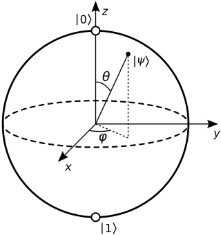
In quantum mechanics and computing, the Bloch sphere is a geometrical representation of the pure state space of a two-level quantum mechanical system (qubit), named after the physicist Felix Bloch.
In theoretical physics, the Bogoliubov transformation, also known as the Bogoliubov–Valatin transformation, was independently developed in 1958 by Nikolay Bogolyubov and John George Valatin for finding solutions of BCS theory in a homogeneous system. The Bogoliubov transformation is an isomorphism of either the canonical commutation relation algebra or canonical anticommutation relation algebra. This induces an autoequivalence on the respective representations. The Bogoliubov transformation is often used to diagonalize Hamiltonians, which yields the stationary solutions of the corresponding Schrödinger equation. The Bogoliubov transformation is also important for understanding the Unruh effect, Hawking radiation, Davies-Fulling radiation, pairing effects in nuclear physics, and many other topics.

In quantum field theory, the Lehmann–Symanzik–Zimmermann (LSZ) reduction formula is a method to calculate S-matrix elements from the time-ordered correlation functions of a quantum field theory. It is a step of the path that starts from the Lagrangian of some quantum field theory and leads to prediction of measurable quantities. It is named after the three German physicists Harry Lehmann, Kurt Symanzik and Wolfhart Zimmermann.
Quantum tomography or quantum state tomography is the process by which a quantum state is reconstructed using measurements on an ensemble of identical quantum states. The source of these states may be any device or system which prepares quantum states either consistently into quantum pure states or otherwise into general mixed states. To be able to uniquely identify the state, the measurements must be tomographically complete. That is, the measured operators must form an operator basis on the Hilbert space of the system, providing all the information about the state. Such a set of observations is sometimes called a quorum. The term tomography was first used in the quantum physics literature in a 1993 paper introducing experimental optical homodyne tomography.
A quasiprobability distribution is a mathematical object similar to a probability distribution but which relaxes some of Kolmogorov's axioms of probability theory. Quasiprobabilities share several of general features with ordinary probabilities, such as, crucially, the ability to yield expectation values with respect to the weights of the distribution. However, they can violate the σ-additivity axiom: integrating over them does not necessarily yield probabilities of mutually exclusive states. Indeed, quasiprobability distributions also have regions of negative probability density, counterintuitively, contradicting the first axiom. Quasiprobability distributions arise naturally in the study of quantum mechanics when treated in phase space formulation, commonly used in quantum optics, time-frequency analysis, and elsewhere.
In quantum physics, the squeeze operator for a single mode of the electromagnetic field is
Nonclassical light is light that cannot be described using classical electromagnetism; its characteristics are described by the quantized electromagnetic field and quantum mechanics.
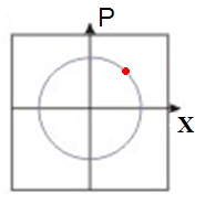
The Glauber–Sudarshan P representation is a suggested way of writing down the phase space distribution of a quantum system in the phase space formulation of quantum mechanics. The P representation is the quasiprobability distribution in which observables are expressed in normal order. In quantum optics, this representation, formally equivalent to several other representations, is sometimes preferred over such alternative representations to describe light in optical phase space, because typical optical observables, such as the particle number operator, are naturally expressed in normal order. It is named after George Sudarshan and Roy J. Glauber, who worked on the topic in 1963. Despite many useful applications in laser theory and coherence theory, the Sudarshan–Glauber P representation has the peculiarity that it is not always positive, and is not a bona-fide probability function.
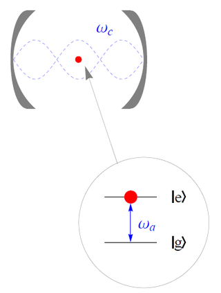
The Jaynes–Cummings model is a theoretical model in quantum optics. It describes the system of a two-level atom interacting with a quantized mode of an optical cavity, with or without the presence of light. It was originally developed to study the interaction of atoms with the quantized electromagnetic field in order to investigate the phenomena of spontaneous emission and absorption of photons in a cavity.
Photon polarization is the quantum mechanical description of the classical polarized sinusoidal plane electromagnetic wave. An individual photon can be described as having right or left circular polarization, or a superposition of the two. Equivalently, a photon can be described as having horizontal or vertical linear polarization, or a superposition of the two.
The Wigner D-matrix is a unitary matrix in an irreducible representation of the groups SU(2) and SO(3). It was introduced in 1927 by Eugene Wigner, and plays a fundamental role in the quantum mechanical theory of angular momentum. The complex conjugate of the D-matrix is an eigenfunction of the Hamiltonian of spherical and symmetric rigid rotors. The letter D stands for Darstellung, which means "representation" in German.
In physics, a quantum amplifier is an amplifier that uses quantum mechanical methods to amplify a signal; examples include the active elements of lasers and optical amplifiers.
Resonance fluorescence is the process in which a two-level atom system interacts with the quantum electromagnetic field if the field is driven at a frequency near to the natural frequency of the atom.
Coherent states have been introduced in a physical context, first as quasi-classical states in quantum mechanics, then as the backbone of quantum optics and they are described in that spirit in the article Coherent states. However, they have generated a huge variety of generalizations, which have led to a tremendous amount of literature in mathematical physics. In this article, we sketch the main directions of research on this line. For further details, we refer to several existing surveys.
In pure and applied mathematics, quantum mechanics and computer graphics, a tensor operator generalizes the notion of operators which are scalars and vectors. A special class of these are spherical tensor operators which apply the notion of the spherical basis and spherical harmonics. The spherical basis closely relates to the description of angular momentum in quantum mechanics and spherical harmonic functions. The coordinate-free generalization of a tensor operator is known as a representation operator.
Phase-space representation of quantum state vectors is a formulation of quantum mechanics elaborating the phase-space formulation with a Hilbert space. It "is obtained within the framework of the relative-state formulation. For this purpose, the Hilbert space of a quantum system is enlarged by introducing an auxiliary quantum system. Relative-position state and relative-momentum state are defined in the extended Hilbert space of the composite quantum system and expressions of basic operators such as canonical position and momentum operators, acting on these states, are obtained." Thus, it is possible to assign a meaning to the wave function in phase space, , as a quasiamplitude, associated to a quasiprobability distribution.
In quantum computing, the variational quantum eigensolver (VQE) is a quantum algorithm for quantum chemistry, quantum simulations and optimization problems. It is a hybrid algorithm that uses both classical computers and quantum computers to find the ground state of a given physical system. Given a guess or ansatz, the quantum processor calculates the expectation value of the system with respect to an observable, often the Hamiltonian, and a classical optimizer is used to improve the guess. The algorithm is based on the variational method of quantum mechanics.


