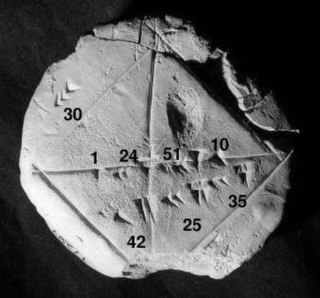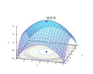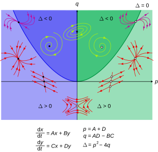
Numerical analysis is the study of algorithms that use numerical approximation for the problems of mathematical analysis. Numerical analysis finds application in all fields of engineering and the physical sciences, and in the 21st century also the life and social sciences, medicine, business and even the arts. Current growth in computing power has enabled the use of more complex numerical analysis, providing detailed and realistic mathematical models in science and engineering. Examples of numerical analysis include: ordinary differential equations as found in celestial mechanics, numerical linear algebra in data analysis, and stochastic differential equations and Markov chains for simulating living cells in medicine and biology.

Mathematical optimization or mathematical programming is the selection of a best element, with regard to some criterion, from some set of available alternatives. Optimization problems of sorts arise in all quantitative disciplines from computer science and engineering to operations research and economics, and the development of solution methods has been of interest in mathematics for centuries.

In mathematics and science, a nonlinear system is a system in which the change of the output is not proportional to the change of the input. Nonlinear problems are of interest to engineers, biologists, physicists, mathematicians, and many other scientists because most systems are inherently nonlinear in nature. Nonlinear dynamical systems, describing changes in variables over time, may appear chaotic, unpredictable, or counterintuitive, contrasting with much simpler linear systems.

In mathematics, an autonomous system or autonomous differential equation is a system of ordinary differential equations which does not explicitly depend on the independent variable. When the variable is time, they are also called time-invariant systems.
Optimal control theory is a branch of mathematical optimization that deals with finding a control for a dynamical system over a period of time such that an objective function is optimized. It has numerous applications in science, engineering and operations research. For example, the dynamical system might be a spacecraft with controls corresponding to rocket thrusters, and the objective might be to reach the moon with minimum fuel expenditure. Or the dynamical system could be a nation's economy, with the objective to minimize unemployment; the controls in this case could be fiscal and monetary policy. A dynamical system may also be introduced to embed operations research problems within the framework of optimal control theory.
In optimal control theory, the Hamilton–Jacobi–Bellman (HJB) equation gives a necessary and sufficient condition for optimality of a control with respect to a loss function. It is, in general, a nonlinear partial differential equation in the value function, which means its solution is the value function itself. Once this solution is known, it can be used to obtain the optimal control by taking the maximizer of the Hamiltonian involved in the HJB equation.
Column generation or delayed column generation is an efficient algorithm for solving large linear programs.
Model predictive control (MPC) is an advanced method of process control that is used to control a process while satisfying a set of constraints. It has been in use in the process industries in chemical plants and oil refineries since the 1980s. In recent years it has also been used in power system balancing models and in power electronics. Model predictive controllers rely on dynamic models of the process, most often linear empirical models obtained by system identification. The main advantage of MPC is the fact that it allows the current timeslot to be optimized, while keeping future timeslots in account. This is achieved by optimizing a finite time-horizon, but only implementing the current timeslot and then optimizing again, repeatedly, thus differing from a linear–quadratic regulator (LQR). Also MPC has the ability to anticipate future events and can take control actions accordingly. PID controllers do not have this predictive ability. MPC is nearly universally implemented as a digital control, although there is research into achieving faster response times with specially designed analog circuitry.
Trajectory optimization is the process of designing a trajectory that minimizes some measure of performance while satisfying a set of constraints. Generally speaking, trajectory optimization is a technique for computing an open-loop solution to an optimal control problem. It is often used for systems where computing the full closed-loop solution is not required, impractical or impossible. If a trajectory optimization problem can be solved at a rate given by the inverse of the Lipschitz constant, then it can be used iteratively to generate a closed-loop solution in the sense of Caratheodory. If only the first step of the trajectory is executed for an infinite-horizon problem, then this is known as Model Predictive Control (MPC).

In mathematics, the relaxation of a (mixed) integer linear program is the problem that arises by removing the integrality constraint of each variable.
Sequential quadratic programming (SQP) is an iterative method for constrained nonlinear optimization. SQP methods are used on mathematical problems for which the objective function and the constraints are twice continuously differentiable.

In mathematical optimization, a feasible region, feasible set, search space, or solution space is the set of all possible points of an optimization problem that satisfy the problem's constraints, potentially including inequalities, equalities, and integer constraints. This is the initial set of candidate solutions to the problem, before the set of candidates has been narrowed down.
The TOMLAB Optimization Environment is a modeling platform for solving applied optimization problems in MATLAB.
Multi-objective optimization is an area of multiple criteria decision making that is concerned with mathematical optimization problems involving more than one objective function to be optimized simultaneously. Multi-objective optimization has been applied in many fields of science, including engineering, economics and logistics where optimal decisions need to be taken in the presence of trade-offs between two or more conflicting objectives. Minimizing cost while maximizing comfort while buying a car, and maximizing performance whilst minimizing fuel consumption and emission of pollutants of a vehicle are examples of multi-objective optimization problems involving two and three objectives, respectively. In practical problems, there can be more than three objectives.
Advanced process monitor (APMonitor) is a modeling language for differential algebraic (DAE) equations. It is a free web-service or local server for solving representations of physical systems in the form of implicit DAE models. APMonitor is suited for large-scale problems and solves linear programming, integer programming, nonlinear programming, nonlinear mixed integer programming, dynamic simulation, moving horizon estimation, and nonlinear model predictive control. APMonitor does not solve the problems directly, but calls nonlinear programming solvers such as APOPT, BPOPT, IPOPT, MINOS, and SNOPT. The APMonitor API provides exact first and second derivatives of continuous functions to the solvers through automatic differentiation and in sparse matrix form.
The Gauss pseudospectral method (GPM), one of many topics named after Carl Friedrich Gauss, is a direct transcription method for discretizing a continuous optimal control problem into a nonlinear program (NLP). The Gauss pseudospectral method differs from several other pseudospectral methods in that the dynamics are not collocated at either endpoint of the time interval. This collocation, in conjunction with the proper approximation to the costate, leads to a set of KKT conditions that are identical to the discretized form of the first-order optimality conditions. This equivalence between the KKT conditions and the discretized first-order optimality conditions leads to an accurate costate estimate using the KKT multipliers of the NLP.
Pseudospectral optimal control is a joint theoretical-computational method for solving optimal control problems. It combines pseudospectral (PS) theory with optimal control theory to produce PS optimal control theory. PS optimal control theory has been used in ground and flight systems in military and industrial applications. The techniques have been extensively used to solve a wide range of problems such as those arising in UAV trajectory generation, missile guidance, control of robotic arms, vibration damping, lunar guidance, magnetic control, swing-up and stabilization of an inverted pendulum, orbit transfers, tether libration control, ascent guidance and quantum control.
In operations research, the Big M method is a method of solving linear programming problems using the simplex algorithm. The Big M method extends the simplex algorithm to problems that contain "greater-than" constraints. It does so by associating the constraints with large negative constants which would not be part of any optimal solution, if it exists.
GPOPS-II is a general-purpose MATLAB software for solving continuous optimal control problems using hp-adaptive Gaussian quadrature collocation and sparse nonlinear programming. The acronym GPOPS stands for "General Purpose OPtimal Control Software", and the Roman numeral "II" refers to the fact that GPOPS-II is the second software of its type.
The GEKKO Python package solves large-scale mixed-integer and differential algebraic equations with nonlinear programming solvers. Modes of operation include machine learning, data reconciliation, real-time optimization, dynamic simulation, and nonlinear model predictive control. In addition, the package solves Linear programming (LP), Quadratic programming (QP), Quadratically constrained quadratic program (QCQP), Nonlinear programming (NLP), Mixed integer programming (MIP), and Mixed integer linear programming (MILP). GEKKO is available in Python and installed with pip from PyPI of the Python Software Foundation.


