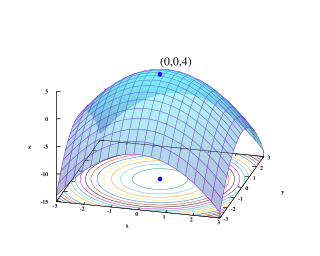
Quadratic programming (QP) is the process of solving certain mathematical optimization problems involving quadratic functions. Specifically, one seeks to optimize a multivariate quadratic function subject to linear constraints on the variables. Quadratic programming is a type of nonlinear programming.

Linear programming (LP), also called linear optimization, is a method to achieve the best outcome in a mathematical model whose requirements and objective are represented by linear relationships. Linear programming is a special case of mathematical programming.
Mathematical optimization or mathematical programming is the selection of a best element, with regard to some criteria, from some set of available alternatives. It is generally divided into two subfields: discrete optimization and continuous optimization. Optimization problems arise in all quantitative disciplines from computer science and engineering to operations research and economics, and the development of solution methods has been of interest in mathematics for centuries.

Optimal control theory is a branch of control theory that deals with finding a control for a dynamical system over a period of time such that an objective function is optimized. It has numerous applications in science, engineering and operations research. For example, the dynamical system might be a spacecraft with controls corresponding to rocket thrusters, and the objective might be to reach the Moon with minimum fuel expenditure. Or the dynamical system could be a nation's economy, with the objective to minimize unemployment; the controls in this case could be fiscal and monetary policy. A dynamical system may also be introduced to embed operations research problems within the framework of optimal control theory.
Multi-disciplinary design optimization (MDO) is a field of engineering that uses optimization methods to solve design problems incorporating a number of disciplines. It is also known as multidisciplinary system design optimization (MSDO), and multidisciplinary design analysis and optimization (MDAO).
In mathematical optimization, the active-set method is an algorithm used to identify the active constraints in a set of inequality constraints. The active constraints are then expressed as equality constraints, thereby transforming an inequality-constrained problem into a simpler equality-constrained subproblem.

In mathematical optimization, the cutting-plane method is any of a variety of optimization methods that iteratively refine a feasible set or objective function by means of linear inequalities, termed cuts. Such procedures are commonly used to find integer solutions to mixed integer linear programming (MILP) problems, as well as to solve general, not necessarily differentiable convex optimization problems. The use of cutting planes to solve MILP was introduced by Ralph E. Gomory.
Interior-point methods are algorithms for solving linear and non-linear convex optimization problems. IPMs combine two advantages of previously-known algorithms:
Convex optimization is a subfield of mathematical optimization that studies the problem of minimizing convex functions over convex sets. Many classes of convex optimization problems admit polynomial-time algorithms, whereas mathematical optimization is in general NP-hard.
In mathematical optimization, the Karush–Kuhn–Tucker (KKT) conditions, also known as the Kuhn–Tucker conditions, are first derivative tests for a solution in nonlinear programming to be optimal, provided that some regularity conditions are satisfied.
The Frank–Wolfe algorithm is an iterative first-order optimization algorithm for constrained convex optimization. Also known as the conditional gradient method, reduced gradient algorithm and the convex combination algorithm, the method was originally proposed by Marguerite Frank and Philip Wolfe in 1956. In each iteration, the Frank–Wolfe algorithm considers a linear approximation of the objective function, and moves towards a minimizer of this linear function.
In mathematical optimization theory, duality or the duality principle is the principle that optimization problems may be viewed from either of two perspectives, the primal problem or the dual problem. If the primal is a minimization problem then the dual is a maximization problem. Any feasible solution to the primal (minimization) problem is at least as large as any feasible solution to the dual (maximization) problem. Therefore, the solution to the primal is an upper bound to the solution of the dual, and the solution of the dual is a lower bound to the solution of the primal. This fact is called weak duality.
In mathematical optimization, constrained optimization is the process of optimizing an objective function with respect to some variables in the presence of constraints on those variables. The objective function is either a cost function or energy function, which is to be minimized, or a reward function or utility function, which is to be maximized. Constraints can be either hard constraints, which set conditions for the variables that are required to be satisfied, or soft constraints, which have some variable values that are penalized in the objective function if, and based on the extent that, the conditions on the variables are not satisfied.
Semidefinite programming (SDP) is a subfield of mathematical programming concerned with the optimization of a linear objective function over the intersection of the cone of positive semidefinite matrices with an affine space, i.e., a spectrahedron.
Penalty methods are a certain class of algorithms for solving constrained optimization problems.

In mathematical optimization and computer science, a feasible region,feasible set, or solution space is the set of all possible points of an optimization problem that satisfy the problem's constraints, potentially including inequalities, equalities, and integer constraints. This is the initial set of candidate solutions to the problem, before the set of candidates has been narrowed down.
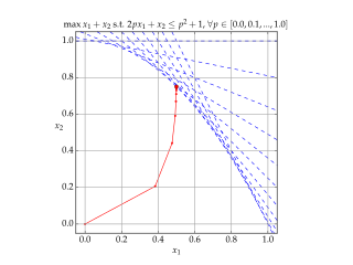
In mathematical optimization, a quadratically constrained quadratic program (QCQP) is an optimization problem in which both the objective function and the constraints are quadratic functions. It has the form
In operations research, the Big M method is a method of solving linear programming problems using the simplex algorithm. The Big M method extends the simplex algorithm to problems that contain "greater-than" constraints. It does so by associating the constraints with large negative constants which would not be part of any optimal solution, if it exists.
Lexicographic max-min optimization is a kind of multi-objective optimization. In general, multi-objective optimization deals with optimization problems with two or more objective functions to be optimized simultaneously. Lexmaxmin optimization presumes that the decision-maker would like the smallest objective value to be as high as possible; subject to this, the second-smallest objective should be as high as possible; and so on. In other words, the decision-maker ranks the possible solutions according to a leximin order of their objective function values.


