
In physics, the Lorentz transformations are a six-parameter family of linear transformations from a coordinate frame in spacetime to another frame that moves at a constant velocity relative to the former. The respective inverse transformation is then parameterized by the negative of this velocity. The transformations are named after the Dutch physicist Hendrik Lorentz.
Quadratic programming (QP) is the process of solving certain mathematical optimization problems involving quadratic functions. Specifically, one seeks to optimize a multivariate quadratic function subject to linear constraints on the variables. Quadratic programming is a type of nonlinear programming.

In probability theory and statistics, the multivariate normal distribution, multivariate Gaussian distribution, or joint normal distribution is a generalization of the one-dimensional (univariate) normal distribution to higher dimensions. One definition is that a random vector is said to be k-variate normally distributed if every linear combination of its k components has a univariate normal distribution. Its importance derives mainly from the multivariate central limit theorem. The multivariate normal distribution is often used to describe, at least approximately, any set of (possibly) correlated real-valued random variables each of which clusters around a mean value.
Ray transfer matrix analysis is a mathematical form for performing ray tracing calculations in sufficiently simple problems which can be solved considering only paraxial rays. Each optical element is described by a 2×2 ray transfer matrix which operates on a vector describing an incoming light ray to calculate the outgoing ray. Multiplication of the successive matrices thus yields a concise ray transfer matrix describing the entire optical system. The same mathematics is also used in accelerator physics to track particles through the magnet installations of a particle accelerator, see electron optics.
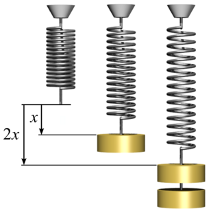
In physics, Hooke's law is an empirical law which states that the force needed to extend or compress a spring by some distance scales linearly with respect to that distance—that is, Fs = kx, where k is a constant factor characteristic of the spring, and x is small compared to the total possible deformation of the spring. The law is named after 17th-century British physicist Robert Hooke. He first stated the law in 1676 as a Latin anagram. He published the solution of his anagram in 1678 as: ut tensio, sic vis. Hooke states in the 1678 work that he was aware of the law since 1660.
In linear algebra, a square matrix is called diagonalizable or non-defective if it is similar to a diagonal matrix, i.e., if there exists an invertible matrix and a diagonal matrix such that , or equivalently . For a finite-dimensional vector space , a linear map is called diagonalizable if there exists an ordered basis of consisting of eigenvectors of . These definitions are equivalent: if has a matrix representation as above, then the column vectors of form a basis consisting of eigenvectors of , and the diagonal entries of are the corresponding eigenvalues of ; with respect to this eigenvector basis, is represented by .Diagonalization is the process of finding the above and .

In linear algebra, a Jordan normal form, also known as a Jordan canonical form or JCF, is an upper triangular matrix of a particular form called a Jordan matrix representing a linear operator on a finite-dimensional vector space with respect to some basis. Such a matrix has each non-zero off-diagonal entry equal to 1, immediately above the main diagonal, and with identical diagonal entries to the left and below them.
In mathematical optimization, Dantzig's simplex algorithm is a popular algorithm for linear programming.
In mathematics and computing, the Levenberg–Marquardt algorithm, also known as the damped least-squares (DLS) method, is used to solve non-linear least squares problems. These minimization problems arise especially in least squares curve fitting. The LMA interpolates between the Gauss–Newton algorithm (GNA) and the method of gradient descent. The LMA is more robust than the GNA, which means that in many cases it finds a solution even if it starts very far off the final minimum. For well-behaved functions and reasonable starting parameters, the LMA tends to be slower than the GNA. LMA can also be viewed as Gauss–Newton using a trust region approach.
In mathematical optimization theory, the linear complementarity problem (LCP) arises frequently in computational mechanics and encompasses the well-known quadratic programming as a special case. It was proposed by Cottle and Dantzig in 1968.
Mehrotra's predictor–corrector method in optimization is a specific interior point method for linear programming. It was proposed in 1989 by Sanjay Mehrotra.

In applied mathematics, in particular the context of nonlinear system analysis, a phase plane is a visual display of certain characteristics of certain kinds of differential equations; a coordinate plane with axes being the values of the two state variables, say, or etc.. It is a two-dimensional case of the general n-dimensional phase space.
In linear algebra, an eigenvector or characteristic vector of a linear transformation is a nonzero vector that changes at most by a scalar factor when that linear transformation is applied to it. The corresponding eigenvalue, often denoted by , is the factor by which the eigenvector is scaled.
In continuum mechanics, a Mooney–Rivlin solid is a hyperelastic material model where the strain energy density function is a linear combination of two invariants of the left Cauchy–Green deformation tensor . The model was proposed by Melvin Mooney in 1940 and expressed in terms of invariants by Ronald Rivlin in 1948.
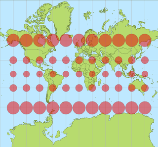
In cartography, a Tissot's indicatrix is a mathematical contrivance presented by French mathematician Nicolas Auguste Tissot in 1859 and 1871 in order to characterize local distortions due to map projection. It is the geometry that results from projecting a circle of infinitesimal radius from a curved geometric model, such as a globe, onto a map. Tissot proved that the resulting diagram is an ellipse whose axes indicate the two principal directions along which scale is maximal and minimal at that point on the map.

Prony analysis was developed by Gaspard Riche de Prony in 1795. However, practical use of the method awaited the digital computer. Similar to the Fourier transform, Prony's method extracts valuable information from a uniformly sampled signal and builds a series of damped complex exponentials or damped sinusoids. This allows for the estimation of frequency, amplitude, phase and damping components of a signal.
In statistics, Bayesian multivariate linear regression is a Bayesian approach to multivariate linear regression, i.e. linear regression where the predicted outcome is a vector of correlated random variables rather than a single scalar random variable. A more general treatment of this approach can be found in the article MMSE estimator.
In linear algebra, eigendecomposition is the factorization of a matrix into a canonical form, whereby the matrix is represented in terms of its eigenvalues and eigenvectors. Only diagonalizable matrices can be factorized in this way. When the matrix being factorized is a normal or real symmetric matrix, the decomposition is called "spectral decomposition", derived from the spectral theorem.

In physics, deformation is the continuum mechanics transformation of a body from a reference configuration to a current configuration. A configuration is a set containing the positions of all particles of the body.
In numerical linear algebra, the conjugate gradient method is an iterative method for numerically solving the linear system


