Quadratic programming (QP) is the process of solving certain mathematical optimization problems involving quadratic functions. Specifically, one seeks to optimize a multivariate quadratic function subject to linear constraints on the variables. Quadratic programming is a type of nonlinear programming.

Linear programming (LP), also called linear optimization, is a method to achieve the best outcome in a mathematical model whose requirements and objective are represented by linear relationships. Linear programming is a special case of mathematical programming.
Gradient descent is a method for unconstrained mathematical optimization. It is a first-order iterative algorithm for minimizing a differentiable multivariate function.

In mathematics, a real-valued function is called convex if the line segment between any two distinct points on the graph of the function lies above or on the graph between the two points. Equivalently, a function is convex if its epigraph is a convex set. In simple terms, a convex function graph is shaped like a cup , while a concave function's graph is shaped like a cap .
In mathematics, Fatou's lemma establishes an inequality relating the Lebesgue integral of the limit inferior of a sequence of functions to the limit inferior of integrals of these functions. The lemma is named after Pierre Fatou.
An integer programming problem is a mathematical optimization or feasibility program in which some or all of the variables are restricted to be integers. In many settings the term refers to integer linear programming (ILP), in which the objective function and the constraints are linear.
Interior-point methods are algorithms for solving linear and non-linear convex optimization problems. IPMs combine two advantages of previously-known algorithms:
Convex optimization is a subfield of mathematical optimization that studies the problem of minimizing convex functions over convex sets. Many classes of convex optimization problems admit polynomial-time algorithms, whereas mathematical optimization is in general NP-hard.
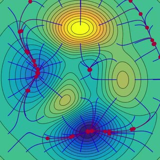
In mathematical optimization, the Karush–Kuhn–Tucker (KKT) conditions, also known as the Kuhn–Tucker conditions, are first derivative tests for a solution in nonlinear programming to be optimal, provided that some regularity conditions are satisfied.
In evolutionary computation, differential evolution (DE) is a method that optimizes a problem by iteratively trying to improve a candidate solution with regard to a given measure of quality. Such methods are commonly known as metaheuristics as they make few or no assumptions about the optimized problem and can search very large spaces of candidate solutions. However, metaheuristics such as DE do not guarantee an optimal solution is ever found.
In mathematical optimization, constrained optimization is the process of optimizing an objective function with respect to some variables in the presence of constraints on those variables. The objective function is either a cost function or energy function, which is to be minimized, or a reward function or utility function, which is to be maximized. Constraints can be either hard constraints, which set conditions for the variables that are required to be satisfied, or soft constraints, which have some variable values that are penalized in the objective function if, and based on the extent that, the conditions on the variables are not satisfied.
In mathematical optimization, the ellipsoid method is an iterative method for minimizing convex functions over convex sets. The ellipsoid method generates a sequence of ellipsoids whose volume uniformly decreases at every step, thus enclosing a minimizer of a convex function.
The cross-entropy (CE) method is a Monte Carlo method for importance sampling and optimization. It is applicable to both combinatorial and continuous problems, with either a static or noisy objective.
In applied mathematics, polyharmonic splines are used for function approximation and data interpolation. They are very useful for interpolating and fitting scattered data in many dimensions. Special cases include thin plate splines and natural cubic splines in one dimension.
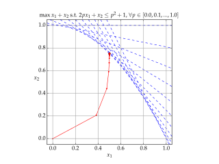
Penalty methods are a certain class of algorithms for solving constrained optimization problems.
Subgradient methods are convex optimization methods which use subderivatives. Originally developed by Naum Z. Shor and others in the 1960s and 1970s, subgradient methods are convergent when applied even to a non-differentiable objective function. When the objective function is differentiable, sub-gradient methods for unconstrained problems use the same search direction as the method of steepest descent.
A self-concordant function is a function satisfying a certain differential inequality, which makes it particularly easy for optimization using Newton's method A self-concordant barrier is a particular self-concordant function, that is also a barrier function for a particular convex set. Self-concordant barriers are important ingredients in interior point methods for optimization.
In mathematics, the logarithmic norm is a real-valued functional on operators, and is derived from either an inner product, a vector norm, or its induced operator norm. The logarithmic norm was independently introduced by Germund Dahlquist and Sergei Lozinskiĭ in 1958, for square matrices. It has since been extended to nonlinear operators and unbounded operators as well. The logarithmic norm has a wide range of applications, in particular in matrix theory, differential equations and numerical analysis. In the finite-dimensional setting, it is also referred to as the matrix measure or the Lozinskiĭ measure.
The dual of a given linear program (LP) is another LP that is derived from the original LP in the following schematic way:
Augmented Lagrangian methods are a certain class of algorithms for solving constrained optimization problems. They have similarities to penalty methods in that they replace a constrained optimization problem by a series of unconstrained problems and add a penalty term to the objective, but the augmented Lagrangian method adds yet another term designed to mimic a Lagrange multiplier. The augmented Lagrangian is related to, but not identical with, the method of Lagrange multipliers.


