In statistics, the Gauss–Markov theorem states that the ordinary least squares (OLS) estimator has the lowest sampling variance within the class of linear unbiased estimators, if the errors in the linear regression model are uncorrelated, have equal variances and expectation value of zero. The errors do not need to be normal for the theorem to apply, nor do they need to be independent and identically distributed.

In probability theory and statistics, a covariance matrix is a square matrix giving the covariance between each pair of elements of a given random vector.
In linear algebra, a Vandermonde matrix, named after Alexandre-Théophile Vandermonde, is a matrix with the terms of a geometric progression in each row: an matrix

In mathematics, a block matrix or a partitioned matrix is a matrix that is interpreted as having been broken into sections called blocks or submatrices.
In numerical linear algebra, a Givens rotation is a rotation in the plane spanned by two coordinates axes. Givens rotations are named after Wallace Givens, who introduced them to numerical analysts in the 1950s while he was working at Argonne National Laboratory.
In linear algebra, linear transformations can be represented by matrices. If is a linear transformation mapping to and is a column vector with entries, then
In electrical engineering and electronics, a network is a collection of interconnected components. Network analysis is the process of finding the voltages across, and the currents through, all network components. There are many techniques for calculating these values; however, for the most part, the techniques assume linear components. Except where stated, the methods described in this article are applicable only to linear network analysis.
In signal processing, the Wiener filter is a filter used to produce an estimate of a desired or target random process by linear time-invariant (LTI) filtering of an observed noisy process, assuming known stationary signal and noise spectra, and additive noise. The Wiener filter minimizes the mean square error between the estimated random process and the desired process.
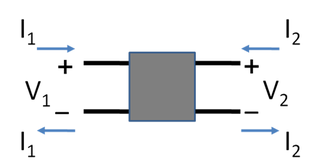
In electronics, a two-port network is an electrical network or device with two pairs of terminals to connect to external circuits. Two terminals constitute a port if the currents applied to them satisfy the essential requirement known as the port condition: the current entering one terminal must equal the current emerging from the other terminal on the same port. The ports constitute interfaces where the network connects to other networks, the points where signals are applied or outputs are taken. In a two-port network, often port 1 is considered the input port and port 2 is considered the output port.
Scattering parameters or S-parameters describe the electrical behavior of linear electrical networks when undergoing various steady state stimuli by electrical signals.

In electric circuits analysis, nodal analysis, node-voltage analysis, or the branch current method is a method of determining the voltage between "nodes" in an electrical circuit in terms of the branch currents.
In power engineering, nodal admittance matrix is an N x N matrix describing a linear power system with N buses. It represents the nodal admittance of the buses in a power system. In realistic systems which contain thousands of buses, the admittance matrix is quite sparse. Each bus in a real power system is usually connected to only a few other buses through the transmission lines. The nodal admittance matrix is used in the formulation of the power flow problem.
Admittance parameters or Y-parameters are properties used in many areas of electrical engineering, such as power, electronics, and telecommunications. These parameters are used to describe the electrical behavior of linear electrical networks. They are also used to describe the small-signal (linearized) response of non-linear networks. Y parameters are also known as short circuited admittance parameters. They are members of a family of similar parameters used in electronic engineering, other examples being: S-parameters, Z-parameters, H-parameters, T-parameters or ABCD-parameters.
Impedance parameters or Z-parameters are properties used in electrical engineering, electronic engineering, and communication systems engineering to describe the electrical behavior of linear electrical networks. They are also used to describe the small-signal (linearized) response of non-linear networks. They are members of a family of similar parameters used in electronic engineering, other examples being: S-parameters, Y-parameters, H-parameters, T-parameters or ABCD-parameters.
An equivalent impedance is an equivalent circuit of an electrical network of impedance elements which presents the same impedance between all pairs of terminals as did the given network. This article describes mathematical transformations between some passive, linear impedance networks commonly found in electronic circuits.
An antimetric electrical network is an electrical network that exhibits anti-symmetrical electrical properties. The term is often encountered in filter theory, but it applies to general electrical network analysis. Antimetric is the diametrical opposite of symmetric; it does not merely mean "asymmetric". It is possible for networks to be symmetric or antimetric in their electrical properties without being physically or topologically symmetric or antimetric.
In control system theory, and various branches of engineering, a transfer function matrix, or just transfer matrix is a generalisation of the transfer functions of single-input single-output (SISO) systems to multiple-input and multiple-output (MIMO) systems. The matrix relates the outputs of the system to its inputs. It is a particularly useful construction for linear time-invariant (LTI) systems because it can be expressed in terms of the s-plane.
In power engineering, Kron reduction is a method used to reduce or eliminate the desired node without need of repeating the steps like in Gaussian elimination.
Performance modelling is the abstraction of a real system into a simplified representation to enable the prediction of performance. The creation of a model can provide insight into how a proposed or actual system will or does work. This can, however, point towards different things to people belonging to different fields of work.

Generalized pencil-of-function method (GPOF), also known as matrix pencil method, is a signal processing technique for estimating a signal or extracting information with complex exponentials. Being similar to Prony and original pencil-of-function methods, it is generally preferred to those for its robustness and computational efficiency.


