This article relies largely or entirely on a single source. Relevant discussion may be found on the talk page. Please help improve this article by introducing citations to additional sources.(November 2009)
In mathematics, the secondary measure associated with a measure of positive density ρ when there is one, is a measure of positive density μ, turning the secondary polynomials associated with the orthogonal polynomials for ρ into an orthogonal system.
In mathematical analysis, a measure on a set is a systematic way to assign a number to each suitable subset of that set, intuitively interpreted as its size. In this sense, a measure is a generalization of the concepts of length, area, and volume. A particularly important example is the Lebesgue measure on a Euclidean space, which assigns the conventional length, area, and volume of Euclidean geometry to suitable subsets of the n-dimensional Euclidean space Rn. For instance, the Lebesgue measure of the interval [0, 1] in the real numbers is its length in the everyday sense of the word, specifically, 1.
The density, or more precisely, the volumetric mass density, of a substance is its mass per unit volume. The symbol most often used for density is ρ, although the Latin letter D can also be used. Mathematically, density is defined as mass divided by volume:
In mathematics, the secondary polynomials associated with a sequence of polynomials orthogonal with respect to a density are defined by
Under certain assumptions that we will specify further, it is possible to obtain the existence of a secondary measure and even to express it.
For example, if one works in the Hilbert spaceL2([0, 1], R, ρ)
The mathematical concept of a Hilbert space, named after David Hilbert, generalizes the notion of Euclidean space. It extends the methods of vector algebra and calculus from the two-dimensional Euclidean plane and three-dimensional space to spaces with any finite or infinite number of dimensions. A Hilbert space is an abstract vector space possessing the structure of an inner product that allows length and angle to be measured. Furthermore, Hilbert spaces are complete: there are enough limits in the space to allow the techniques of calculus to be used.
In mathematics, the Stieltjes transformationSρ(z) of a measure of density ρ on a real interval I is the function of the complex variable z defined outside I by the formula
in which c1 is the moment of order 1 of the measure ρ.
In mathematics, a moment is a specific quantitative measure of the shape of a function. It is used in both mechanics and statistics. If the function represents physical density, then the zeroth moment is the total mass, the first moment divided by the total mass is the center of mass, and the second moment is the rotational inertia. If the function is a probability distribution, then the zeroth moment is the total probability, the first moment is the mean, the second central moment is the variance, the third standardized moment is the skewness, and the fourth standardized moment is the kurtosis. The mathematical concept is closely related to the concept of moment in physics.
These secondary measures, and the theory around them, lead to some surprising results, and make it possible to find in an elegant way quite a few traditional formulas of analysis, mainly around the Euler Gamma function, Riemann Zeta function, and Euler's constant.
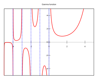
In mathematics, the gamma function is one of a number of extensions of the factorial function with its argument shifted down by 1, to real and complex numbers. Derived by Daniel Bernoulli, if n is a positive integer,
The Riemann zeta function or Euler–Riemann zeta function, ζ(s), is a function of a complex variable s that analytically continues the sum of the Dirichlet series
The Euler–Mascheroni constant is a mathematical constant recurring in analysis and number theory, usually denoted by the lowercase Greek letter gamma.
They also allowed the clarification of integrals and series with a tremendous effectiveness, though it is a priori difficult.
Finally they make it possible to solve integral equations of the form
where g is the unknown function, and lead to theorems of convergence towards the Chebyshev and Dirac measures.
In mathematics, a Dirac measure assigns a size to a set based solely on whether it contains a fixed element x or not. It is one way of formalizing the idea of the Dirac delta function, an important tool in physics and other technical fields.
The broad outlines of the theory
Let ρ be a measure of positive density on an interval I and admitting moments of any order. We can build a family {Pn} of orthogonal polynomials for the inner product induced by ρ. Let us call {Qn} the sequence of the secondary polynomials associated with the family P. Under certain conditions there is a measure for which the family Q is orthogonal. This measure, which we can clarify from ρ is called a secondary measure associated initial measure ρ.
When ρ is a probability density function, a sufficient condition so that μ, while admitting moments of any order can be a secondary measure associated with ρ is that its Stieltjes Transformation is given by an equality of the type:
a is an arbitrary constant and c1 indicating the moment of order 1 of ρ.
For a = 1 we obtain the measure known as secondary, remarkable since for n ≥ 1 the norm of the polynomial Pn for ρ coincides exactly with the norm of the secondary polynomial associated Qn when using the measure μ.
In this paramount case, and if the space generated by the orthogonal polynomials is dense in L2(I, R, ρ), the operatorTρ defined by
creating the secondary polynomials can be furthered to a linear map connecting space L2(I, R, ρ) to L2(I, R, μ) and becomes isometric if limited to the hyperplaneHρ of the orthogonal functions with P0 = 1.
The theory continues by introducing the concept of reducible measure, meaning that the quotient ρ/μ is element of L2(I, R, μ). The following results are then established:
The reducer φ of ρ is an antecedent of ρ/μ for the operator Tρ. (In fact the only antecedent which belongs to Hρ).
For any function square integrable for ρ, there is an equality known as the reducing formula:
.
The operator
defined on the polynomials is prolonged in an isometrySρ linking the closure of the space of these polynomials in L2(I, R, ρ2μ−1) to the hyperplaneHρ provided with the norm induced by ρ.
Under certain restrictive conditions the operator Sρ acts like the adjoint of Tρ for the inner product induced by ρ.
Finally the two operators are also connected, provided the images in question are defined, by the fundamental formula of composition:
Case of the Lebesgue measure and some other examples
The Lebesgue measure on the standard interval [0, 1] is obtained by taking the constant density ρ(x) = 1.
The recurrence relation in three terms is written:
The reducer of this measure of Lebesgue is given by
The associated secondary measure is then clarified as
.
If we normalize the polynomials of Legendre, the coefficients of Fourier of the reducer φ related to this orthonormal system are null for an even index and are given by
for an odd index n.
The Laguerre polynomials are linked to the density ρ(x) = e−x on the interval I = [0, ∞). They are clarified by
and are normalized.
The reducer associated is defined by
The coefficients of Fourier of the reducer φ related to the Laguerre polynomials are given by
This coefficient Cn(φ) is no other than the opposite of the sum of the elements of the line of index n in the table of the harmonic triangular numbers of Leibniz.
The coefficients of Fourier of the reducer φ related to the system of Hermite polynomials are null for an even index and are given by
for an odd index n.
The Chebyshev measure of the second form. This is defined by the density
on the interval [0, 1].
It is the only one which coincides with its secondary measure normalised on this standard interval. Under certain conditions it occurs as the limit of the sequence of normalized secondary measures of a given density.
Examples of non-reducible measures
Jacobi measure on (0, 1) of density
Chebyshev measure on (−1,1) of the first form of density
Sequence of secondary measures
The secondary measure μ associated with a probability density function ρ has its moment of order 0 given by the formula
where c1 and c2 indicating the respective moments of order 1 and 2 of ρ.
To be able to iterate the process then, one 'normalizes' μ while defining ρ1 = μ/d0 which becomes in its turn a density of probability called naturally the normalised secondary measure associated with ρ.
We can then create from ρ1 a secondary normalised measure ρ2, then defining ρ3 from ρ2 and so on. We can therefore see a sequence of successive secondary measures, created from ρ0 = ρ, is such that ρn+1 that is the secondary normalised measure deduced from ρn
It is possible to clarify the density ρn by using the orthogonal polynomialsPn for ρ, the secondary polynomials Qn and the reducer associated φ. That gives the formula
The coefficient is easily obtained starting from the leading coefficients of the polynomials Pn−1 and Pn. We can also clarify the reducer φn associated with ρn, as well as the orthogonal polynomials corresponding to ρn.
A very beautiful result relates the evolution of these densities when the index tends towards the infinite and the support of the measure is the standard interval [0, 1].
Let
be the classic recurrence relation in three terms. If
then the sequence {ρn} converges completely towards the Chebyshev density of the second form
.
These conditions about limits are checked by a very broad class of traditional densities. A derivation of the sequence of secondary measures and convergence can be found in [1]
Equinormal measures
One calls two measures thus leading to the same normalised secondary density. It is remarkable that the elements of a given class and having the same moment of order 1 are connected by a homotopy. More precisely, if the density function ρ has its moment of order 1 equal to c1, then these densities equinormal with ρ are given by a formula of the type:
t describing an interval containing ]0, 1].
If μ is the secondary measure of ρ, that of ρt will be tμ.
The reducer of ρt is
by noting G(x) the reducer of μ.
Orthogonal polynomials for the measure ρt are clarified from n = 1 by the formula
with Qn secondary polynomial associated with Pn.
It is remarkable also that, within the meaning of distributions, the limit when t tends towards 0 per higher value of ρt is the Dirac measure concentrated at c1.
For example, the equinormal densities with the Chebyshev measure of the second form are defined by:
with t describing ]0, 2]. The value t = 2 gives the Chebyshev measure of the first form.
The notation indicating the 2 periodic function coinciding with on (−1, 1).
If the measure ρ is reducible and let φ be the associated reducer, one has the equality
If the measure ρ is reducible with μ the associated reducer, then if f is square integrable for μ, and if g is square integrable for ρ and is orthogonal with P0 = 1 one has equivalence:
c1 indicates the moment of order 1 of ρ and Tρ the operator
In addition, the sequence of secondary measures has applications in Quantum Mechanics. The sequence gives rise to the so-called sequence of residual spectral densities for specialized Pauli-Fierz Hamiltonians. This also provides a physical interpretation for the sequence of secondary measures. [1]
In mathematics, the Dirac delta function is a generalized function or distribution introduced by the physicist Paul Dirac. It is used to model the density of an idealized point mass or point charge as a function equal to zero everywhere except for zero and whose integral over the entire real line is equal to one. As there is no function that has these properties, the computations made by the theoretical physicists appeared to mathematicians as nonsense until the introduction of distributions by Laurent Schwartz to formalize and validate the computations. As a distribution, the Dirac delta function is a linear functional that maps every function to its value at zero. The Kronecker delta function, which is usually defined on a discrete domain and takes values 0 and 1, is a discrete analog of the Dirac delta function.
In mathematics, the prime-counting function is the function counting the number of prime numbers less than or equal to some real number x. It is denoted by π(x).
The concept of a normalizing constant arises in probability theory and a variety of other areas of mathematics. The normalizing constant is used to reduce any probability function to a probability density function with total probability of one.
In the theory of stochastic processes, the Karhunen–Loève theorem, also known as the Kosambi–Karhunen–Loève theorem is a representation of a stochastic process as an infinite linear combination of orthogonal functions, analogous to a Fourier series representation of a function on a bounded interval. The transformation is also known as Hotelling transform and eigenvector transform, and is closely related to principal component analysis (PCA) technique widely used in image processing and in data analysis in many fields.
In probability theory, a distribution is said to be stable if a linear combination of two independent random variables with this distribution has the same distribution, up to location and scale parameters. A random variable is said to be stable if its distribution is stable. The stable distribution family is also sometimes referred to as the Lévy alpha-stable distribution, after Paul Lévy, the first mathematician to have studied it.
In statistics and signal processing, an autoregressive (AR) model is a representation of a type of random process; as such, it is used to describe certain time-varying processes in nature, economics, etc. The autoregressive model specifies that the output variable depends linearly on its own previous values and on a stochastic term ; thus the model is in the form of a stochastic difference equation. In machine learning, an autoregressive model learns from a series of timed steps and takes measurements from previous actions as inputs for a regression model, in order to predict the value of the next time step.
In Bayesian probability, the Jeffreys prior, named after Sir Harold Jeffreys, is a non-informative (objective) prior distribution for a parameter space; it is proportional to the square root of the determinant of the Fisher information matrix:
In mathematics, the Zernike polynomials are a sequence of polynomials that are orthogonal on the unit disk. Named after optical physicist Frits Zernike, winner of the 1953 Nobel Prize in Physics and the inventor of phase-contrast microscopy, they play an important role in beam optics.
In mathematics, the explicit formulae for L-functions are relations between sums over the complex number zeroes of an L-function and sums over prime powers, introduced by Riemann (1859) for the Riemann zeta function. Such explicit formulae have been applied also to questions on bounding the discriminant of an algebraic number field, and the conductor of a number field.
The multiple integral is a definite integral of a function of more than one real variable, for example, f(x, y) or f(x, y, z). Integrals of a function of two variables over a region in R2 are called double integrals, and integrals of a function of three variables over a region of R3 are called triple integrals.
In probability theory, calculation of the sum of normally distributed random variables is an instance of the arithmetic of random variables, which can be quite complex based on the probability distributions of the random variables involved and their relationships.
In probability theory and statistics, the characteristic function of any real-valued random variable completely defines its probability distribution. If a random variable admits a probability density function, then the characteristic function is the Fourier transform of the probability density function. Thus it provides the basis of an alternative route to analytical results compared with working directly with probability density functions or cumulative distribution functions. There are particularly simple results for the characteristic functions of distributions defined by the weighted sums of random variables.
The Wigner distribution function (WDF) is used in signal processing as a transform in time-frequency analysis.
Cylindrical multipole moments are the coefficients in a series expansion of a potential that varies logarithmically with the distance to a source, i.e., as . Such potentials arise in the electric potential of long line charges, and the analogous sources for the magnetic potential and gravitational potential.
In electrodynamics, the retarded potentials are the electromagnetic potentials for the electromagnetic field generated by time-varying electric current or charge distributions in the past. The fields propagate at the speed of light c, so the delay of the fields connecting cause and effect at earlier and later times is an important factor: the signal takes a finite time to propagate from a point in the charge or current distribution to another point in space, see figure below.
In fluid dynamics, the Oseen equations describe the flow of a viscous and incompressible fluid at small Reynolds numbers, as formulated by Carl Wilhelm Oseen in 1910. Oseen flow is an improved description of these flows, as compared to Stokes flow, with the (partial) inclusion of convective acceleration.
In probability theory and directional statistics, a wrapped normal distribution is a wrapped probability distribution that results from the "wrapping" of the normal distribution around the unit circle. It finds application in the theory of Brownian motion and is a solution to the heat equation for periodic boundary conditions. It is closely approximated by the von Mises distribution, which, due to its mathematical simplicity and tractability, is the most commonly used distribution in directional statistics.
Lagrangian field theory is a formalism in classical field theory. It is the field-theoretic analogue of Lagrangian mechanics. Lagrangian mechanics is used for discrete particles each with a finite number of degrees of freedom. Lagrangian field theory applies to continua and fields, which have an infinite number of degrees of freedom.
References
1 2 Mappings of open quantum systems onto chain representations and Markovian embeddings, M. P. Woods, R. Groux, A. W. Chin, S. F. Huelga, M. B. Plenio. https://arxiv.org/abs/1111.5262
This page is based on this Wikipedia article Text is available under the CC BY-SA 4.0 license; additional terms may apply. Images, videos and audio are available under their respective licenses.