Nonlinear dimensionality reduction, also known as manifold learning, is any of various related techniques that aim to project high-dimensional data, potentially existing across non-linear manifolds which cannot be adequately captured by linear decomposition methods, onto lower-dimensional latent manifolds, with the goal of either visualizing the data in the low-dimensional space, or learning the mapping itself. The techniques described below can be understood as generalizations of linear decomposition methods used for dimensionality reduction, such as singular value decomposition and principal component analysis.

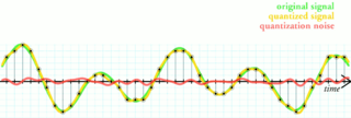
Quantization, in mathematics and digital signal processing, is the process of mapping input values from a large set to output values in a (countable) smaller set, often with a finite number of elements. Rounding and truncation are typical examples of quantization processes. Quantization is involved to some degree in nearly all digital signal processing, as the process of representing a signal in digital form ordinarily involves rounding. Quantization also forms the core of essentially all lossy compression algorithms.
Latent semantic analysis (LSA) is a technique in natural language processing, in particular distributional semantics, of analyzing relationships between a set of documents and the terms they contain by producing a set of concepts related to the documents and terms. LSA assumes that words that are close in meaning will occur in similar pieces of text. A matrix containing word counts per document is constructed from a large piece of text and a mathematical technique called singular value decomposition (SVD) is used to reduce the number of rows while preserving the similarity structure among columns. Documents are then compared by cosine similarity between any two columns. Values close to 1 represent very similar documents while values close to 0 represent very dissimilar documents.
Wireless sensor networks (WSNs) refer to networks of spatially dispersed and dedicated sensors that monitor and record the physical conditions of the environment and forward the collected data to a central location. WSNs can measure environmental conditions such as temperature, sound, pollution levels, humidity and wind.
The scale-invariant feature transform (SIFT) is a computer vision algorithm to detect, describe, and match local features in images, invented by David Lowe in 1999. Applications include object recognition, robotic mapping and navigation, image stitching, 3D modeling, gesture recognition, video tracking, individual identification of wildlife and match moving.

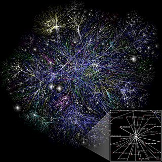
In graph theory and network analysis, indicators of centrality assign numbers or rankings to nodes within a graph corresponding to their network position. Applications include identifying the most influential person(s) in a social network, key infrastructure nodes in the Internet or urban networks, super-spreaders of disease, and brain networks. Centrality concepts were first developed in social network analysis, and many of the terms used to measure centrality reflect their sociological origin.
Recurrent neural networks (RNNs) are a class of artificial neural network commonly used for sequential data processing. Unlike feedforward neural networks, which process data in a single pass, RNNs process data across multiple time steps, making them well-adapted for modelling and processing text, speech, and time series.
In computer networking, linear network coding is a program in which intermediate nodes transmit data from source nodes to sink nodes by means of linear combinations.
The structural similarityindex measure (SSIM) is a method for predicting the perceived quality of digital television and cinematic pictures, as well as other kinds of digital images and videos. It is also used for measuring the similarity between two images. The SSIM index is a full reference metric; in other words, the measurement or prediction of image quality is based on an initial uncompressed or distortion-free image as reference.
Machine olfaction is the automated simulation of the sense of smell. An emerging application in modern engineering, it involves the use of robots or other automated systems to analyze air-borne chemicals. Such an apparatus is often called an electronic nose or e-nose. The development of machine olfaction is complicated by the fact that e-nose devices to date have responded to a limited number of chemicals, whereas odors are produced by unique sets of odorant compounds. The technology, though still in the early stages of development, promises many applications, such as: quality control in food processing, detection and diagnosis in medicine, detection of drugs, explosives and other dangerous or illegal substances, disaster response, and environmental monitoring.

Long short-term memory (LSTM) is a type of recurrent neural network (RNN) aimed at mitigating the vanishing gradient problem commonly encountered by traditional RNNs. Its relative insensitivity to gap length is its advantage over other RNNs, hidden Markov models, and other sequence learning methods. It aims to provide a short-term memory for RNN that can last thousands of timesteps. The name is made in analogy with long-term memory and short-term memory and their relationship, studied by cognitive psychologists since the early 20th century.
Mean shift is a non-parametric feature-space mathematical analysis technique for locating the maxima of a density function, a so-called mode-seeking algorithm. Application domains include cluster analysis in computer vision and image processing.
Compressed sensing is a signal processing technique for efficiently acquiring and reconstructing a signal, by finding solutions to underdetermined linear systems. This is based on the principle that, through optimization, the sparsity of a signal can be exploited to recover it from far fewer samples than required by the Nyquist–Shannon sampling theorem. There are two conditions under which recovery is possible. The first one is sparsity, which requires the signal to be sparse in some domain. The second one is incoherence, which is applied through the isometric property, which is sufficient for sparse signals. Compressed sensing has applications in, for example, MRI where the incoherence condition is typically satisfied.
Location estimation in wireless sensor networks is the problem of estimating the location of an object from a set of noisy measurements. These measurements are acquired in a distributed manner by a set of sensors.
In the mathematical theory of artificial neural networks, universal approximation theorems are theorems of the following form: Given a family of neural networks, for each function from a certain function space, there exists a sequence of neural networks from the family, such that according to some criterion. That is, the family of neural networks is dense in the function space.
The Brooks–Iyengar algorithm or FuseCPA Algorithm or Brooks–Iyengar hybrid algorithm is a distributed algorithm that improves both the precision and accuracy of the interval measurements taken by a distributed sensor network, even in the presence of faulty sensors. The sensor network does this by exchanging the measured value and accuracy value at every node with every other node, and computes the accuracy range and a measured value for the whole network from all of the values collected. Even if some of the data from some of the sensors is faulty, the sensor network will not malfunction. The algorithm is fault-tolerant and distributed. It could also be used as a sensor fusion method. The precision and accuracy bound of this algorithm have been proved in 2016.

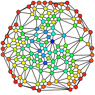
In graph theory, betweenness centrality is a measure of centrality in a graph based on shortest paths. For every pair of vertices in a connected graph, there exists at least one shortest path between the vertices such that either the number of edges that the path passes through or the sum of the weights of the edges is minimized. The betweenness centrality for each vertex is the number of these shortest paths that pass through the vertex.
Extreme learning machines are feedforward neural networks for classification, regression, clustering, sparse approximation, compression and feature learning with a single layer or multiple layers of hidden nodes, where the parameters of hidden nodes need to be tuned. These hidden nodes can be randomly assigned and never updated, or can be inherited from their ancestors without being changed. In most cases, the output weights of hidden nodes are usually learned in a single step, which essentially amounts to learning a linear model.

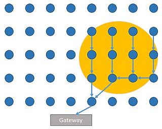
Wireless sensor networks (WSN) are a spatially distributed network of autonomous sensors used for monitoring an environment. Energy cost is a major limitation for WSN requiring the need for energy efficient networks and processing. One of major energy costs in WSN is the energy spent on communication between nodes and it is sometimes desirable to only send data to a gateway node when an event of interest is triggered at a sensor. Sensors will then only open communication during a probable event, saving on communication costs. Fields interested in this type of network include surveillance, home automation, disaster relief, traffic control, health care and more.
A graph neural network (GNN) belongs to a class of artificial neural networks for processing data that can be represented as graphs.


