Spectral leakage

The Fourier transform of a function of time, s(t), is a complex-valued function of frequency, S(f), often referred to as a frequency spectrum. Any linear time-invariant operation on s(t) produces a new spectrum of the form H(f)•S(f), which changes the relative magnitudes and/or angles (phase) of the non-zero values of S(f). Any other type of operation creates new frequency components that may be referred to as spectral leakage in the broadest sense. Sampling, for instance, produces leakage, which we call aliases of the original spectral component. For Fourier transform purposes, sampling is modeled as a product between s(t) and a Dirac comb function. The spectrum of a product is the convolution between S(f) and another function, which inevitably creates the new frequency components. But the term 'leakage' usually refers to the effect of windowing, which is the product of s(t) with a different kind of function, the window function. Window functions happen to have finite duration, but that is not necessary to create leakage. Multiplication by a time-variant function is sufficient.

Spectral analysis

The Fourier transform of the function cos(ωt) is zero, except at frequency ±ω. However, many other functions and waveforms do not have convenient closed-form transforms. Alternatively, one might be interested in their spectral content only during a certain time period. In either case, the Fourier transform (or a similar transform) can be applied on one or more finite intervals of the waveform. In general, the transform is applied to the product of the waveform and a window function. Any window (including rectangular) affects the spectral estimate computed by this method.

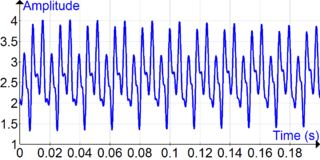
The effects are most easily characterized by their effect on a sinusoidal s(t) function, whose unwindowed Fourier transform is zero for all but one frequency. The customary frequency of choice is 0 Hz, because the windowed Fourier transform is simply the Fourier transform of the window function itself (see § Examples of window functions):

${\displaystyle {\mathcal {F}}\{w(t)\cdot \underbrace {\cos(2\pi 0t)} _{1}\}={\mathcal {F}}\{w(t)\}.}$

When both sampling and windowing are applied to s(t), in either order, the leakage caused by windowing is a relatively localized spreading of frequency components, with often a blurring effect, whereas the aliasing caused by sampling is a periodic repetition of the entire blurred spectrum.

Figure 1: Comparison of two window functions in terms of their effects on equal-strength sinusoids with additive noise. The sinusoid at bin −20 suffers no scalloping and the one at bin +20.5 exhibits worst-case scalloping. The rectangular window produces the most scalloping but also narrower peaks and lower noise-floor. A third sinusoid with amplitude −16 dB would be noticeable in the upper spectrum, but not in the lower spectrum.

Figure 2: Windowing a sinusoid causes spectral leakage, even if the sinusoid has an integer number of cycles within a rectangular window. The leakage is evident in the 2nd row, blue trace. It is the same amount as the red trace, which represents a slightly higher frequency that does not have an integer number of cycles. When the sinusoid is sampled and windowed, its discrete-time Fourier transform also exhibits the same leakage pattern (rows 3 and 4). But when the DTFT is only sparsely sampled, at a certain interval, it is possible (depending on your point of view) to: (1) avoid the leakage, or (2) create the illusion of no leakage. For the case of the blue sinusoid DTFT (3rd row of plots, right-hand side), those samples are the outputs of the discrete Fourier transform (DFT). The red sinusoid DTFT (4th row) has the same interval of zero-crossings, but the DFT samples fall in-between them, and the leakage is revealed.

Choice of window function

Windowing of a simple waveform like cos(ωt) causes its Fourier transform to develop non-zero values (commonly called spectral leakage) at frequencies other than ω. The leakage tends to be worst (highest) near ω and least at frequencies farthest from ω.

If the waveform under analysis comprises two sinusoids of different frequencies, leakage can interfere with our ability to distinguish them spectrally. Possible types of interference are often broken down into two opposing classes as follows: If the component frequencies are dissimilar and one component is weaker, then leakage from the stronger component can obscure the weaker one's presence. But if the frequencies are too similar, leakage can render them unresolvable even when the sinusoids are of equal strength. Windows that are effective against the first type of interference, namely where components have dissimilar frequencies and amplitudes, are called high dynamic range . Conversely, windows that can distinguish components with similar frequencies and amplitudes are called high resolution.

The rectangular window is an example of a window that is high resolution but low dynamic range, meaning it is good for distinguishing components of similar amplitude even when the frequencies are also close, but poor at distinguishing components of different amplitude even when the frequencies are far away. High-resolution, low-dynamic-range windows such as the rectangular window also have the property of high sensitivity, which is the ability to reveal relatively weak sinusoids in the presence of additive random noise. That is because the noise produces a stronger response with high-dynamic-range windows than with high-resolution windows.

At the other extreme of the range of window types are windows with high dynamic range but low resolution and sensitivity. High-dynamic-range windows are most often justified in wideband applications, where the spectrum being analyzed is expected to contain many different components of various amplitudes.

In between the extremes are moderate windows, such as Hann and Hamming. They are commonly used in narrowband applications, such as the spectrum of a telephone channel.

In summary, spectral analysis involves a trade-off between resolving comparable strength components with similar frequencies (high resolution / sensitivity) and resolving disparate strength components with dissimilar frequencies (high dynamic range). That trade-off occurs when the window function is chosen. ^{[1] : p.90}

Discrete-time signals

When the input waveform is time-sampled, instead of continuous, the analysis is usually done by applying a window function and then a discrete Fourier transform (DFT). But the DFT provides only a sparse sampling of the actual discrete-time Fourier transform (DTFT) spectrum. Figure 2, row 3 shows a DTFT for a rectangularly-windowed sinusoid. The actual frequency of the sinusoid is indicated as "13" on the horizontal axis. Everything else is leakage, exaggerated by the use of a logarithmic presentation. The unit of frequency is "DFT bins"; that is, the integer values on the frequency axis correspond to the frequencies sampled by the DFT. ^{[2] : p.56 eq.(16)} So the figure depicts a case where the actual frequency of the sinusoid coincides with a DFT sample, and the maximum value of the spectrum is accurately measured by that sample. In row 4, it misses the maximum value by 1⁄2 bin, and the resultant measurement error is referred to as scalloping loss (inspired by the shape of the peak). For a known frequency, such as a musical note or a sinusoidal test signal, matching the frequency to a DFT bin can be prearranged by choices of a sampling rate and a window length that results in an integer number of cycles within the window.

Figure 3: This figure compares the processing losses of three window functions for sinusoidal inputs, with both minimum and maximum scalloping loss.

Noise bandwidth

The concepts of resolution and dynamic range tend to be somewhat subjective, depending on what the user is actually trying to do. But they also tend to be highly correlated with the total leakage, which is quantifiable. It is usually expressed as an equivalent bandwidth, B. It can be thought of as redistributing the DTFT into a rectangular shape with height equal to the spectral maximum and width B. ^{[upper-alpha 1] [3]} The more the leakage, the greater the bandwidth. It is sometimes called noise equivalent bandwidth or equivalent noise bandwidth, because it is proportional to the average power that will be registered by each DFT bin when the input signal contains a random noise component (or is just random noise). A graph of the power spectrum, averaged over time, typically reveals a flat noise floor , caused by this effect. The height of the noise floor is proportional to B. So two different window functions can produce different noise floors, as seen in figures 1 and 3.

Processing gain and losses

In signal processing, operations are chosen to improve some aspect of quality of a signal by exploiting the differences between the signal and the corrupting influences. When the signal is a sinusoid corrupted by additive random noise, spectral analysis distributes the signal and noise components differently, often making it easier to detect the signal's presence or measure certain characteristics, such as amplitude and frequency. Effectively, the signal-to-noise ratio (SNR) is improved by distributing the noise uniformly, while concentrating most of the sinusoid's energy around one frequency. Processing gain is a term often used to describe an SNR improvement. The processing gain of spectral analysis depends on the window function, both its noise bandwidth (B) and its potential scalloping loss. These effects partially offset, because windows with the least scalloping naturally have the most leakage.

Figure 3 depicts the effects of three different window functions on the same data set, comprising two equal strength sinusoids in additive noise. The frequencies of the sinusoids are chosen such that one encounters no scalloping and the other encounters maximum scalloping. Both sinusoids suffer less SNR loss under the Hann window than under the Blackman-Harris window. In general (as mentioned earlier), this is a deterrent to using high-dynamic-range windows in low-dynamic-range applications.

Figure 4: Two different ways to generate an 8-point Gaussian window sequence (σ = 0.4) for spectral analysis applications. MATLAB calls them "symmetric" and "periodic". The latter is also historically called DFT-even.

Figure 5: Spectral leakage characteristics of the functions in Figure 4

Symmetry

The formulas provided at § Examples of window functions produce discrete sequences, as if a continuous window function has been "sampled". (See an example at Kaiser window.) Window sequences for spectral analysis are either symmetric or 1-sample short of symmetric (called periodic, ^{[4] [5]} DFT-even, or DFT-symmetric ^{[2] : p.52}). For instance, a true symmetric sequence, with its maximum at a single center-point, is generated by the MATLAB function hann(9,'symmetric'). Deleting the last sample produces a sequence identical to hann(8,'periodic'). Similarly, the sequence hann(8,'symmetric') has two equal center-points. ^[6]

Some functions have one or two zero-valued end-points, which are unnecessary in most applications. Deleting a zero-valued end-point has no effect on its DTFT (spectral leakage). But the function designed for N + 1 or N + 2 samples, in anticipation of deleting one or both end points, typically has a slightly narrower main lobe, slightly higher sidelobes, and a slightly smaller noise-bandwidth. ^[7]

DFT-symmetry

The predecessor of the DFT is the finite Fourier transform, and window functions were "always an odd number of points and exhibit even symmetry about the origin". ^{[2] : p.52} In that case, the DTFT is entirely real-valued. When the same sequence is shifted into a DFT data window, ${\displaystyle [0\leq n\leq N],}$ the DTFT becomes complex-valued except at frequencies spaced at regular intervals of ${\displaystyle 1/N.}$ ^{[lower-alpha 1]} Thus, when sampled by an ${\displaystyle N}$-length DFT, the samples (called DFT coefficients) are still real-valued. An approximation is to truncate the N+1-length sequence (effectively ${\displaystyle w[N]=0}$), and compute an ${\displaystyle N}$-length DFT. The DTFT (spectral leakage) is slightly affected, but the samples remain real-valued. ^{[8] [upper-alpha 2]} The terms DFT-even and periodic refer to the idea that if the truncated sequence were repeated periodically, it would be even-symmetric about ${\displaystyle n=0,}$ and its DTFT would be entirely real-valued. But the actual DTFT is generally complex-valued, except for the ${\displaystyle N}$ DFT coefficients. Spectral plots like those at § Examples of window functions, are produced by sampling the DTFT at much smaller intervals than ${\displaystyle 1/N}$ and displaying only the magnitude component of the complex numbers.

Periodic summation

An exact method to sample the DTFT of an N+1-length sequence at intervals of ${\displaystyle 1/N}$ is described at DTFT § L=N+1. Essentially, ${\displaystyle w[N]}$ is combined with ${\displaystyle w[0]}$ (by addition), and an ${\displaystyle N}$-point DFT is done on the truncated sequence. Similarly, spectral analysis would be done by combining the ${\displaystyle n=0}$ and ${\displaystyle n=N}$ data samples before applying the truncated symmetric window. That is not a common practice, even though truncated windows are very popular. ^{[2] [9] [10] [11] [12] [13] [lower-alpha 2]}

Convolution

The appeal of DFT-symmetric windows is explained by the popularity of the fast Fourier transform (FFT) algorithm for implementation of the DFT, because truncation of an odd-length sequence results in an even-length sequence. Their real-valued DFT coefficients are also an advantage in certain esoteric applications ^{[upper-alpha 3]} where windowing is achieved by means of convolution between the DFT coefficients and an unwindowed DFT of the data. ^{[14] [2] : p.62  [1] : p.85} In those applications, DFT-symmetric windows (even or odd length) from the Cosine-sum family are preferred, because most of their DFT coefficients are zero-valued, making the convolution very efficient. ^{[upper-alpha 4] [1] : p.85}

Some window metrics

Comparison of spectral leakage of several window functions

When selecting an appropriate window function for an application, this comparison graph may be useful. The frequency axis has units of FFT "bins" when the window of length N is applied to data and a transform of length N is computed. For instance, the value at frequency ⁠1/2⁠ "bin" is the response that would be measured in bins k and k + 1 to a sinusoidal signal at frequency k + ⁠1/2⁠. It is relative to the maximum possible response, which occurs when the signal frequency is an integer number of bins. The value at frequency ⁠1/2⁠ is referred to as the maximum scalloping loss of the window, which is one metric used to compare windows. The rectangular window is noticeably worse than the others in terms of that metric.

Other metrics that can be seen are the width of the main lobe and the peak level of the sidelobes, which respectively determine the ability to resolve comparable strength signals and disparate strength signals. The rectangular window (for instance) is the best choice for the former and the worst choice for the latter. What cannot be seen from the graphs is that the rectangular window has the best noise bandwidth, which makes it a good candidate for detecting low-level sinusoids in an otherwise white noise environment. Interpolation techniques, such as zero-padding and frequency-shifting, are available to mitigate its potential scalloping loss.

See also

• § Sampling the DTFT
• Knife-edge effect, spatial analog of truncation
• Gibbs phenomenon

Notes

1. Mathematically, the noise equivalent bandwidth of transfer function H is the bandwidth of an ideal rectangular filter with the same peak gain as H that would pass the same power with white noise input. In the units of frequency f (e.g. hertz), it is given by:

   ${\displaystyle B_{\text{noise}}={\frac {1}{|H(f)|_{\max }^{2}}}\int _{0}^{\infty }|H(f)|^{2}df.}$

2. An example of the effect of truncation on spectral leakage is figure Gaussian windows. The graph labeled DTFT periodic8 is the DTFT of the truncated window labeled periodic DFT-even (both blue). The green graph labeled DTFT symmetric9 corresponds to the same window with its symmetry restored. The DTFT samples, labeled DFT8 periodic summation, are an example of using periodic summation to sample it at the same frequencies as the blue graph.
3. Sometimes both a windowed and an unwindowed (rectangularly windowed) DFT are needed.
4. For example, see figures DFT-even Hann window and Odd-length, DFT-even Hann window, which show that the ${\displaystyle N}$-length DFT of the sequence generated by hann(${\displaystyle N}$,'periodic') has only three non-zero values. All the other samples coincide with zero-crossings of the DTFT.

Page citations

1. Harris 1978, p.52, where ${\displaystyle \Delta \omega \triangleq 2\pi \Delta f.}$
2. Nuttall 1981, p.85 (15a).

References

1. Nuttall, Albert H. (Feb 1981). "Some Windows with Very Good Sidelobe Behavior". IEEE Transactions on Acoustics, Speech, and Signal Processing. 29 (1): 84–91. doi:10.1109/TASSP.1981.1163506.Extends Harris' paper, covering all the window functions known at the time, along with key metric comparisons.
2. Harris, Fredric J. (Jan 1978). "On the use of Windows for Harmonic Analysis with the Discrete Fourier Transform" (PDF). Proceedings of the IEEE. 66 (1): 51–83. Bibcode:1978IEEEP..66...51H. CiteSeerX   10.1.1.649.9880 . doi:10.1109/PROC.1978.10837. S2CID   426548.The fundamental 1978 paper on FFT windows by Harris, which specified many windows and introduced key metrics used to compare them.
3. Carlson, A. Bruce (1986). Communication Systems: An Introduction to Signals and Noise in Electrical Communication. McGraw-Hill. ISBN   978-0-07-009960-9.
4. "Hann (Hanning) window - MATLAB hann". www.mathworks.com. Retrieved 2020-02-12.
5. "Window Function". www.mathworks.com. Retrieved 2019-04-14.
6. Robertson, Neil (18 December 2018). "Evaluate Window Functions for the Discrete Fourier Transform". DSPRelated.com. The Related Media Group. Retrieved 9 August 2020. Revised 22 February 2020.
7. "Matlab for the Hann Window". ccrma.stanford.edu. Retrieved 2020-09-01.
8. Rohling, H.; Schuermann, J. (March 1983). "Discrete time window functions with arbitrarily low sidelobe level". Signal Processing. 5 (2). Forschungsinstitut Ulm, Sedanstr, Germany: AEG-Telefunken: 127–138. Bibcode:1983SigPr...5..127R. doi:10.1016/0165-1684(83)90019-1 . Retrieved 8 August 2020. It can be shown, that the DFT-even sampling technique as proposed by Harris is not the most suitable one.
9. Heinzel, G.; Rüdiger, A.; Schilling, R. (2002). Spectrum and spectral density estimation by the Discrete Fourier transform (DFT), including a comprehensive list of window functions and some new flat-top windows (Technical report). Max Planck Institute (MPI) für Gravitationsphysik / Laser Interferometry & Gravitational Wave Astronomy. 395068.0. Retrieved 2013-02-10. Also available at https://pure.mpg.de/rest/items/item_152164_1/component/file_152163/content
10. Lyons, Richard (1 June 1998). "Windowing Functions Improve FFT Results". EDN. Sunnyvale, CA: TRW. Retrieved 8 August 2020.
11. Fulton, Trevor (4 March 2008). "DP Numeric Transform Toolbox". herschel.esac.esa.int. Herschel Data Processing. Retrieved 8 August 2020.
12. Poularikas, A.D. (1999). "7.3.1". In Poularikas, Alexander D. (ed.). The Handbook of Formulas and Tables for Signal Processing (PDF). Boca Raton: CRC Press LLC. ISBN   0849385792 . Retrieved 8 August 2020. Windows are even (about the origin) sequences with an odd number of points. The right-most point of the window will be discarded.
13. Puckette, Miller (30 December 2006). "Fourier analysis of non-periodic signals". msp.ucsd.edu. UC San Diego. Retrieved 9 August 2020.
14. USpatent 6898235,Carlin,Joe; Collins,Terry& Hays,Peteret al.,"Wideband communication intercept and direction finding device using hyperchannelization",published 1999-12-10,issued 2005-05-24 , also available at https://patentimages.storage.googleapis.com/4d/39/2a/cec2ae6f33c1e7/US6898235.pdf