In classical mechanics, a harmonic oscillator is a system that, when displaced from its equilibrium position, experiences a restoring force F proportional to the displacement x:

In mathematical analysis, the Dirac delta function, also known as the unit impulse, is a generalized function on the real numbers, whose value is zero everywhere except at zero, and whose integral over the entire real line is equal to one. Since there is no function having this property, to model the delta "function" rigorously involves the use of limits or, as is common in mathematics, measure theory and the theory of distributions.
In vector calculus, the divergence theorem, also known as Gauss's theorem or Ostrogradsky's theorem, is a theorem relating the flux of a vector field through a closed surface to the divergence of the field in the volume enclosed.
In mathematics, a Gaussian function, often simply referred to as a Gaussian, is a function of the base form
In mathematical analysis, Fubini's theorem is a result that gives conditions under which it is possible to compute a double integral by using an iterated integral, introduced by Guido Fubini in 1907. It states that if a function is integrable on a rectangle , then one can evaluate the double integral as an iterated integral:
In mathematical analysis, a function of bounded variation, also known as BV function, is a real-valued function whose total variation is bounded (finite): the graph of a function having this property is well behaved in a precise sense. For a continuous function of a single variable, being of bounded variation means that the distance along the direction of the y-axis, neglecting the contribution of motion along x-axis, traveled by a point moving along the graph has a finite value. For a continuous function of several variables, the meaning of the definition is the same, except for the fact that the continuous path to be considered cannot be the whole graph of the given function, but can be every intersection of the graph itself with a hyperplane parallel to a fixed x-axis and to the y-axis.
In mathematics and signal processing, the Hilbert transform is a specific singular integral that takes a function, u(t) of a real variable and produces another function of a real variable H(u)(t). The Hilbert transform is given by the Cauchy principal value of the convolution with the function (see § Definition). The Hilbert transform has a particularly simple representation in the frequency domain: It imparts a phase shift of ±90° (π/2 radians) to every frequency component of a function, the sign of the shift depending on the sign of the frequency (see § Relationship with the Fourier transform). The Hilbert transform is important in signal processing, where it is a component of the analytic representation of a real-valued signal u(t). The Hilbert transform was first introduced by David Hilbert in this setting, to solve a special case of the Riemann–Hilbert problem for analytic functions.
In mathematics, Laplace's method, named after Pierre-Simon Laplace, is a technique used to approximate integrals of the form
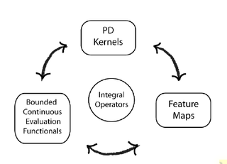
In functional analysis, a reproducing kernel Hilbert space (RKHS) is a Hilbert space of functions in which point evaluation is a continuous linear functional. Roughly speaking, this means that if two functions and in the RKHS are close in norm, i.e., is small, then and are also pointwise close, i.e., is small for all . The converse does not need to be true. Informally, this can be shown by looking at the supremum norm: the sequence of functions converges pointwise, but does not converge uniformly i.e. does not converge with respect to the supremum norm.
In mathematics, Parseval's theorem usually refers to the result that the Fourier transform is unitary; loosely, that the sum of the square of a function is equal to the sum of the square of its transform. It originates from a 1799 theorem about series by Marc-Antoine Parseval, which was later applied to the Fourier series. It is also known as Rayleigh's energy theorem, or Rayleigh's identity, after John William Strutt, Lord Rayleigh.

In mathematics, Monte Carlo integration is a technique for numerical integration using random numbers. It is a particular Monte Carlo method that numerically computes a definite integral. While other algorithms usually evaluate the integrand at a regular grid, Monte Carlo randomly chooses points at which the integrand is evaluated. This method is particularly useful for higher-dimensional integrals.

The Friedmann equations, also known as the Friedmann-Lemaître or FL equations, are a set of equations in physical cosmology that govern the expansion of space in homogeneous and isotropic models of the universe within the context of general relativity. They were first derived by Alexander Friedmann in 1922 from Einstein's field equations of gravitation for the Friedmann–Lemaître–Robertson–Walker metric and a perfect fluid with a given mass density ρ and pressure p. The equations for negative spatial curvature were given by Friedmann in 1924.

The rectangular function is defined as

In quantum field theory, the Lehmann–Symanzik–Zimmermann (LSZ) reduction formula is a method to calculate S-matrix elements from the time-ordered correlation functions of a quantum field theory. It is a step of the path that starts from the Lagrangian of some quantum field theory and leads to prediction of measurable quantities. It is named after the three German physicists Harry Lehmann, Kurt Symanzik and Wolfhart Zimmermann.
In mathematics, a change of variables is a basic technique used to simplify problems in which the original variables are replaced with functions of other variables. The intent is that when expressed in new variables, the problem may become simpler, or equivalent to a better understood problem.
In calculus, the Leibniz integral rule for differentiation under the integral sign states that for an integral of the form
In mathematics, a locally integrable function is a function which is integrable on every compact subset of its domain of definition. The importance of such functions lies in the fact that their function space is similar to Lp spaces, but its members are not required to satisfy any growth restriction on their behavior at the boundary of their domain : in other words, locally integrable functions can grow arbitrarily fast at the domain boundary, but are still manageable in a way similar to ordinary integrable functions.
In the mathematical field of geometric measure theory, the coarea formula expresses the integral of a function over an open set in Euclidean space in terms of integrals over the level sets of another function. A special case is Fubini's theorem, which says under suitable hypotheses that the integral of a function over the region enclosed by a rectangular box can be written as the iterated integral over the level sets of the coordinate functions. Another special case is integration in spherical coordinates, in which the integral of a function on Rn is related to the integral of the function over spherical shells: level sets of the radial function. The formula plays a decisive role in the modern study of isoperimetric problems.
In mathematics, the method of steepest descent or saddle-point method is an extension of Laplace's method for approximating an integral, where one deforms a contour integral in the complex plane to pass near a stationary point, in roughly the direction of steepest descent or stationary phase. The saddle-point approximation is used with integrals in the complex plane, whereas Laplace’s method is used with real integrals.


