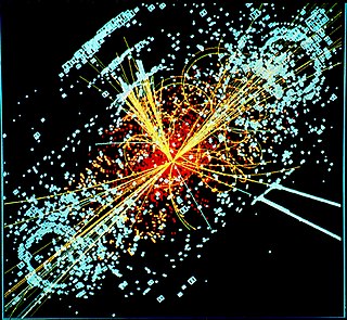
In particle physics, the Dirac equation is a relativistic wave equation derived by British physicist Paul Dirac in 1928. In its free form, or including electromagnetic interactions, it describes all spin-1⁄2 massive particles, called "Dirac particles", such as electrons and quarks for which parity is a symmetry. It is consistent with both the principles of quantum mechanics and the theory of special relativity, and was the first theory to account fully for special relativity in the context of quantum mechanics. It was validated by accounting for the fine structure of the hydrogen spectrum in a completely rigorous way.

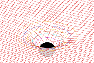
The stress–energy tensor, sometimes called the stress–energy–momentum tensor or the energy–momentum tensor, is a tensor physical quantity that describes the density and flux of energy and momentum in spacetime, generalizing the stress tensor of Newtonian physics. It is an attribute of matter, radiation, and non-gravitational force fields. This density and flux of energy and momentum are the sources of the gravitational field in the Einstein field equations of general relativity, just as mass density is the source of such a field in Newtonian gravity.

In the mathematical field of differential geometry, the Riemann curvature tensor or Riemann–Christoffel tensor is the most common way used to express the curvature of Riemannian manifolds. It assigns a tensor to each point of a Riemannian manifold. It is a local invariant of Riemannian metrics which measures the failure of the second covariant derivatives to commute. A Riemannian manifold has zero curvature if and only if it is flat, i.e. locally isometric to the Euclidean space. The curvature tensor can also be defined for any pseudo-Riemannian manifold, or indeed any manifold equipped with an affine connection.
In physics, Ginzburg–Landau theory, often called Landau–Ginzburg theory, named after Vitaly Ginzburg and Lev Landau, is a mathematical physical theory used to describe superconductivity. In its initial form, it was postulated as a phenomenological model which could describe type-I superconductors without examining their microscopic properties. One GL-type superconductor is the famous YBCO, and generally all Cuprates.

In the theory of partial differential equations, elliptic operators are differential operators that generalize the Laplace operator. They are defined by the condition that the coefficients of the highest-order derivatives be positive, which implies the key property that the principal symbol is invertible, or equivalently that there are no real characteristic directions.
In physics, the Hamilton–Jacobi equation, named after William Rowan Hamilton and Carl Gustav Jacob Jacobi, is an alternative formulation of classical mechanics, equivalent to other formulations such as Newton's laws of motion, Lagrangian mechanics and Hamiltonian mechanics. The Hamilton–Jacobi equation is particularly useful in identifying conserved quantities for mechanical systems, which may be possible even when the mechanical problem itself cannot be solved completely.
In mathematical analysis a pseudo-differential operator is an extension of the concept of differential operator. Pseudo-differential operators are used extensively in the theory of partial differential equations and quantum field theory, e.g. in mathematical models that include ultrametric pseudo-differential equations in a non-Archimedean space.
In differential geometry, the Einstein tensor is used to express the curvature of a pseudo-Riemannian manifold. In general relativity, it occurs in the Einstein field equations for gravitation that describe spacetime curvature in a manner that is consistent with conservation of energy and momentum.
In physics, the Polyakov action is an action of the two-dimensional conformal field theory describing the worldsheet of a string in string theory. It was introduced by Stanley Deser and Bruno Zumino and independently by L. Brink, P. Di Vecchia and P. S. Howe in 1976, and has become associated with Alexander Polyakov after he made use of it in quantizing the string in 1981. The action reads
When studying and formulating Albert Einstein's theory of general relativity, various mathematical structures and techniques are utilized. The main tools used in this geometrical theory of gravitation are tensor fields defined on a Lorentzian manifold representing spacetime. This article is a general description of the mathematics of general relativity.

In probability theory, the Rice distribution or Rician distribution is the probability distribution of the magnitude of a circularly-symmetric bivariate normal random variable, possibly with non-zero mean (noncentral). It was named after Stephen O. Rice (1907–1986).
In differential geometry and mathematical physics, a spin connection is a connection on a spinor bundle. It is induced, in a canonical manner, from the affine connection. It can also be regarded as the gauge field generated by local Lorentz transformations. In some canonical formulations of general relativity, a spin connection is defined on spatial slices and can also be regarded as the gauge field generated by local rotations.
In physics, Maxwell's equations in curved spacetime govern the dynamics of the electromagnetic field in curved spacetime or where one uses an arbitrary coordinate system. These equations can be viewed as a generalization of the vacuum Maxwell's equations which are normally formulated in the local coordinates of flat spacetime. But because general relativity dictates that the presence of electromagnetic fields induce curvature in spacetime, Maxwell's equations in flat spacetime should be viewed as a convenient approximation.

Oblate spheroidal coordinates are a three-dimensional orthogonal coordinate system that results from rotating the two-dimensional elliptic coordinate system about the non-focal axis of the ellipse, i.e., the symmetry axis that separates the foci. Thus, the two foci are transformed into a ring of radius in the x-y plane. Oblate spheroidal coordinates can also be considered as a limiting case of ellipsoidal coordinates in which the two largest semi-axes are equal in length.
In mathematics — specifically, in stochastic analysis — the infinitesimal generator of a Feller process is a Fourier multiplier operator that encodes a great deal of information about the process. The generator is used in evolution equations such as the Kolmogorov backward equation ; its L2 Hermitian adjoint is used in evolution equations such as the Fokker–Planck equation.
In the theory of partial differential equations, Holmgren's uniqueness theorem, or simply Holmgren's theorem, named after the Swedish mathematician Erik Albert Holmgren (1873–1943), is a uniqueness result for linear partial differential equations with real analytic coefficients.
In mathematics, Ricci calculus constitutes the rules of index notation and manipulation for tensors and tensor fields on a differentiable manifold, with or without a metric tensor or connection. It is also the modern name for what used to be called the absolute differential calculus, developed by Gregorio Ricci-Curbastro in 1887–1896, and subsequently popularized in a paper written with his pupil Tullio Levi-Civita in 1900. Jan Arnoldus Schouten developed the modern notation and formalism for this mathematical framework, and made contributions to the theory, during its applications to general relativity and differential geometry in the early twentieth century.
Affine gauge theory is classical gauge theory where gauge fields are affine connections on the tangent bundle over a smooth manifold . For instance, these are gauge theory of dislocations in continuous media when , the generalization of metric-affine gravitation theory when is a world manifold and, in particular, gauge theory of the fifth force.
Lagrangian field theory is a formalism in classical field theory. It is the field-theoretic analogue of Lagrangian mechanics. Lagrangian mechanics is used to analyze the motion of a system of discrete particles each with a finite number of degrees of freedom. Lagrangian field theory applies to continua and fields, which have an infinite number of degrees of freedom.
Attempts have been made to describe gauge theories in terms of extended objects such as Wilson loops and holonomies. The loop representation is a quantum hamiltonian representation of gauge theories in terms of loops. The aim of the loop representation in the context of Yang–Mills theories is to avoid the redundancy introduced by Gauss gauge symmetries allowing to work directly in the space of physical states. The idea is well known in the context of lattice Yang–Mills theory. Attempts to explore the continuous loop representation was made by Gambini and Trias for canonical Yang–Mills theory, however there were difficulties as they represented singular objects. As we shall see the loop formalism goes far beyond a simple gauge invariant description, in fact it is the natural geometrical framework to treat gauge theories and quantum gravity in terms of their fundamental physical excitations.


