Kinematics

"Kinematic" redirects here. For the Australian band, see Kinematic (band).

Kinematics is a subfield of physics, developed in classical mechanics, that describes the motion of points, bodies (objects), and systems of bodies (groups of objects) without considering the forces that cause them to move. ^{[1] [2] [3]} Kinematics, as a field of study, is often referred to as the "geometry of motion" and is occasionally seen as a branch of mathematics. ^{[4] [5] [6]} A kinematics problem begins by describing the geometry of the system and declaring the initial conditions of any known values of position, velocity and/or acceleration of points within the system. Then, using arguments from geometry, the position, velocity and acceleration of any unknown parts of the system can be determined. The study of how forces act on bodies falls within kinetics, not kinematics. For further details, see analytical dynamics.

Kinematics is used in astrophysics to describe the motion of celestial bodies and collections of such bodies. In mechanical engineering, robotics, and biomechanics, ^[7] kinematics is used to describe the motion of systems composed of joined parts (multi-link systems) such as an engine, a robotic arm or the human skeleton.

Geometric transformations, also called rigid transformations, are used to describe the movement of components in a mechanical system, simplifying the derivation of the equations of motion. They are also central to dynamic analysis.

Kinematic analysis is the process of measuring the kinematic quantities used to describe motion. In engineering, for instance, kinematic analysis may be used to find the range of movement for a given mechanism and, working in reverse, using kinematic synthesis to design a mechanism for a desired range of motion. ^[8] In addition, kinematics applies algebraic geometry to the study of the mechanical advantage of a mechanical system or mechanism.

Etymology

The term kinematic is the English version of A.M. Ampère's cinématique, ^[9] which he constructed from the Greek κίνημαkinema ("movement, motion"), itself derived from κινεῖνkinein ("to move"). ^{[10] [11]}

Kinematic and cinématique are related to the French word cinéma, but neither are directly derived from it. However, they do share a root word in common, as cinéma came from the shortened form of cinématographe, "motion picture projector and camera", once again from the Greek word for movement and from the Greek γρᾰ́φωgrapho ("to write"). ^[12]

Kinematics of a particle trajectory in a non-rotating frame of reference

Kinematic quantities of a classical particle: mass m, position r, velocity v, acceleration a.

Position vector r, always points radially from the origin.

Velocity vector v, always tangent to the path of motion.

Acceleration vector a, not parallel to the radial motion but offset by the angular and Coriolis accelerations, nor tangent to the path but offset by the centripetal and radial accelerations.

Kinematic vectors in plane polar coordinates. Notice the setup is not restricted to 2-d space, but a plane in any higher dimension.

Particle kinematics is the study of the trajectory of particles. The position of a particle is defined as the coordinate vector from the origin of a coordinate frame to the particle. For example, consider a tower 50 m south from your home, where the coordinate frame is centered at your home, such that east is in the direction of the x-axis and north is in the direction of the y-axis, then the coordinate vector to the base of the tower is r = (0 m, −50 m, 0 m). If the tower is 50 m high, and this height is measured along the z-axis, then the coordinate vector to the top of the tower is r = (0 m, −50 m, 50 m).

In the most general case, a three-dimensional coordinate system is used to define the position of a particle. However, if the particle is constrained to move within a plane, a two-dimensional coordinate system is sufficient. All observations in physics are incomplete without being described with respect to a reference frame.

The position vector of a particle is a vector drawn from the origin of the reference frame to the particle. It expresses both the distance of the point from the origin and its direction from the origin. In three dimensions, the position vector ${\displaystyle {\bf {r}}}$ can be expressed as

$${\displaystyle \mathbf {r} =(x,y,z)=x{\hat {\mathbf {x} }}+y{\hat {\mathbf {y} }}+z{\hat {\mathbf {z} }},}$$

where ${\displaystyle x}$, ${\displaystyle y}$, and ${\displaystyle z}$ are the Cartesian coordinates and ${\displaystyle {\hat {\mathbf {x} }}}$, ${\displaystyle {\hat {\mathbf {y} }}}$ and ${\displaystyle {\hat {\mathbf {z} }}}$ are the unit vectors along the ${\displaystyle x}$, ${\displaystyle y}$, and ${\displaystyle z}$ coordinate axes, respectively. The magnitude of the position vector ${\displaystyle \left|\mathbf {r} \right|}$ gives the distance between the point ${\displaystyle \mathbf {r} }$ and the origin.

$${\displaystyle |\mathbf {r} |={\sqrt {x^{2}+y^{2}+z^{2}}}.}$$

The direction cosines of the position vector provide a quantitative measure of direction. In general, an object's position vector will depend on the frame of reference; different frames will lead to different values for the position vector.

The trajectory of a particle is a vector function of time, ${\displaystyle \mathbf {r} (t)}$, which defines the curve traced by the moving particle, given by

$${\displaystyle \mathbf {r} (t)=x(t){\hat {\mathbf {x} }}+y(t){\hat {\mathbf {y} }}+z(t){\hat {\mathbf {z} }},}$$

where ${\displaystyle x(t)}$, ${\displaystyle y(t)}$, and ${\displaystyle z(t)}$ describe each coordinate of the particle's position as a function of time.

The distance travelled is always greater than or equal to the displacement.

Velocity and speed

The velocity of a particle is a vector quantity that describes the direction as well as the magnitude of motion of the particle. More mathematically, the rate of change of the position vector of a point with respect to time is the velocity of the point. Consider the ratio formed by dividing the difference of two positions of a particle (displacement) by the time interval. This ratio is called the average velocity over that time interval and is defined as

$${\displaystyle \mathbf {\bar {v}} ={\frac {\Delta \mathbf {r} }{\Delta t}}={\frac {\Delta x}{\Delta t}}{\hat {\mathbf {x} }}+{\frac {\Delta y}{\Delta t}}{\hat {\mathbf {y} }}+{\frac {\Delta z}{\Delta t}}{\hat {\mathbf {z} }}={\bar {v}}_{x}{\hat {\mathbf {x} }}+{\bar {v}}_{y}{\hat {\mathbf {y} }}+{\bar {v}}_{z}{\hat {\mathbf {z} }}\,}$$

where ${\displaystyle \Delta \mathbf {r} }$ is the displacement vector during the time interval ${\displaystyle \Delta t}$. In the limit that the time interval ${\displaystyle \Delta t}$ approaches zero, the average velocity approaches the instantaneous velocity, defined as the time derivative of the position vector,

$${\displaystyle \mathbf {v} =\lim _{\Delta t\to 0}{\frac {\Delta \mathbf {r} }{\Delta t}}={\frac {{\text{d}}\mathbf {r} }{{\text{d}}t}}=v_{x}{\hat {\mathbf {x} }}+v_{y}{\hat {\mathbf {y} }}+v_{z}{\hat {\mathbf {z} }}.}$$

Thus, a particle's velocity is the time rate of change of its position. Furthermore, this velocity is tangent to the particle's trajectory at every position along its path. In a non-rotating frame of reference, the derivatives of the coordinate directions are not considered as their directions and magnitudes are constants.

The speed of an object is the magnitude of its velocity. It is a scalar quantity:

$${\displaystyle v=|\mathbf {v} |={\frac {{\text{d}}s}{{\text{d}}t}},}$$

where ${\displaystyle s}$ is the arc-length measured along the trajectory of the particle. This arc-length must always increase as the particle moves. Hence, ${\displaystyle {\text{d}}s/{\text{d}}t}$ is non-negative, which implies that speed is also non-negative.

Acceleration

The velocity vector can change in magnitude and in direction or both at once. Hence, the acceleration accounts for both the rate of change of the magnitude of the velocity vector and the rate of change of direction of that vector. The same reasoning used with respect to the position of a particle to define velocity, can be applied to the velocity to define acceleration. The acceleration of a particle is the vector defined by the rate of change of the velocity vector. The average acceleration of a particle over a time interval is defined as the ratio.

$${\displaystyle \mathbf {\bar {a}} ={\frac {\Delta \mathbf {\bar {v}} }{\Delta t}}={\frac {\Delta {\bar {v}}_{x}}{\Delta t}}{\hat {\mathbf {x} }}+{\frac {\Delta {\bar {v}}_{y}}{\Delta t}}{\hat {\mathbf {y} }}+{\frac {\Delta {\bar {v}}_{z}}{\Delta t}}{\hat {\mathbf {z} }}={\bar {a}}_{x}{\hat {\mathbf {x} }}+{\bar {a}}_{y}{\hat {\mathbf {y} }}+{\bar {a}}_{z}{\hat {\mathbf {z} }}\,}$$

where Δv is the average velocity and Δt is the time interval.

The acceleration of the particle is the limit of the average acceleration as the time interval approaches zero, which is the time derivative,

$${\displaystyle \mathbf {a} =\lim _{\Delta t\to 0}{\frac {\Delta \mathbf {v} }{\Delta t}}={\frac {{\text{d}}\mathbf {v} }{{\text{d}}t}}=a_{x}{\hat {\mathbf {x} }}+a_{y}{\hat {\mathbf {y} }}+a_{z}{\hat {\mathbf {z} }}.}$$

Alternatively,

$${\displaystyle \mathbf {a} =\lim _{(\Delta t)^{2}\to 0}{\frac {\Delta \mathbf {r} }{(\Delta t)^{2}}}={\frac {{\text{d}}^{2}\mathbf {r} }{{\text{d}}t^{2}}}=a_{x}{\hat {\mathbf {x} }}+a_{y}{\hat {\mathbf {y} }}+a_{z}{\hat {\mathbf {z} }}.}$$

Thus, acceleration is the first derivative of the velocity vector and the second derivative of the position vector of that particle. In a non-rotating frame of reference, the derivatives of the coordinate directions are not considered as their directions and magnitudes are constants.

The magnitude of the acceleration of an object is the magnitude |a| of its acceleration vector. It is a scalar quantity:

$${\displaystyle |\mathbf {a} |=|{\dot {\mathbf {v} }}|={\frac {{\text{d}}v}{{\text{d}}t}}.}$$

Relative position vector

A relative position vector is a vector that defines the position of one point relative to another. It is the difference in position of the two points. The position of one point A relative to another point B is simply the difference between their positions

${\displaystyle \mathbf {r} _{A/B}=\mathbf {r} _{A}-\mathbf {r} _{B}}$

which is the difference between the components of their position vectors.

If point A has position components ${\displaystyle \mathbf {r} _{A}=\left(x_{A},y_{A},z_{A}\right)}$

and point B has position components ${\displaystyle \mathbf {r} _{B}=\left(x_{B},y_{B},z_{B}\right)}$

then the position of point A relative to point B is the difference between their components: ${\displaystyle \mathbf {r} _{A/B}=\mathbf {r} _{A}-\mathbf {r} _{B}=\left(x_{A}-x_{B},y_{A}-y_{B},z_{A}-z_{B}\right)}$

Relative velocity

Main article: Relative velocity

Relative velocities between two particles in classical mechanics.

The velocity of one point relative to another is simply the difference between their velocities

$${\displaystyle \mathbf {v} _{A/B}=\mathbf {v} _{A}-\mathbf {v} _{B}}$$

which is the difference between the components of their velocities.

If point A has velocity components ${\displaystyle \mathbf {v} _{A}=\left(v_{A_{x}},v_{A_{y}},v_{A_{z}}\right)}$ and point B has velocity components ${\displaystyle \mathbf {v} _{B}=\left(v_{B_{x}},v_{B_{y}},v_{B_{z}}\right)}$ then the velocity of point A relative to point B is the difference between their components: ${\displaystyle \mathbf {v} _{A/B}=\mathbf {v} _{A}-\mathbf {v} _{B}=\left(v_{A_{x}}-v_{B_{x}},v_{A_{y}}-v_{B_{y}},v_{A_{z}}-v_{B_{z}}\right)}$

Alternatively, this same result could be obtained by computing the time derivative of the relative position vector r_B/A.

Relative acceleration

The acceleration of one point C relative to another point B is simply the difference between their accelerations.

$${\displaystyle \mathbf {a} _{C/B}=\mathbf {a} _{C}-\mathbf {a} _{B}}$$

which is the difference between the components of their accelerations.

If point C has acceleration components ${\displaystyle \mathbf {a} _{C}=\left(a_{C_{x}},a_{C_{y}},a_{C_{z}}\right)}$ and point B has acceleration components ${\displaystyle \mathbf {a} _{B}=\left(a_{B_{x}},a_{B_{y}},a_{B_{z}}\right)}$ then the acceleration of point C relative to point B is the difference between their components: ${\displaystyle \mathbf {a} _{C/B}=\mathbf {a} _{C}-\mathbf {a} _{B}=\left(a_{C_{x}}-a_{B_{x}},a_{C_{y}}-a_{B_{y}},a_{C_{z}}-a_{B_{z}}\right)}$

Alternatively, this same result could be obtained by computing the second time derivative of the relative position vector r_B/A. ^[13]

Assuming that the initial conditions of the position, ${\displaystyle \mathbf {r} _{0}}$, and velocity ${\displaystyle \mathbf {v} _{0}}$ at time ${\displaystyle t=0}$ are known, the first integration yields the velocity of the particle as a function of time. ^{[lower-alpha 1]}

$${\displaystyle \mathbf {v} (t)=\mathbf {v} _{0}+\int _{0}^{t}\mathbf {a} \,{\text{d}}\tau =\mathbf {v} _{0}+\mathbf {a} t.}$$

A second integration yields its path (trajectory),

$${\displaystyle \mathbf {r} (t)=\mathbf {r} _{0}+\int _{0}^{t}\mathbf {v} (\tau )\,{\text{d}}\tau =\mathbf {r} _{0}+\int _{0}^{t}\left(\mathbf {v} _{0}+\mathbf {a} \tau \right){\text{d}}\tau =\mathbf {r} _{0}+\mathbf {v} _{0}t+{\tfrac {1}{2}}\mathbf {a} t^{2}.}$$

Additional relations between displacement, velocity, acceleration, and time can be derived. Since the acceleration is constant,

$${\displaystyle \mathbf {a} ={\frac {\Delta \mathbf {v} }{\Delta t}}={\frac {\mathbf {v} -\mathbf {v} _{0}}{t}}}$$

can be substituted into the above equation to give:

$${\displaystyle \mathbf {r} (t)=\mathbf {r} _{0}+\left({\frac {\mathbf {v} +\mathbf {v} _{0}}{2}}\right)t.}$$

A relationship between velocity, position and acceleration without explicit time dependence can be had by solving the average acceleration for time and substituting and simplifying

$${\displaystyle t={\frac {\mathbf {v} -\mathbf {v} _{0}}{\mathbf {a} }}}$$

$${\displaystyle \left(\mathbf {r} -\mathbf {r} _{0}\right)\cdot \mathbf {a} =\left(\mathbf {v} -\mathbf {v} _{0}\right)\cdot {\frac {\mathbf {v} +\mathbf {v} _{0}}{2}}\ ,}$$

where ${\displaystyle \cdot }$ denotes the dot product, which is appropriate as the products are scalars rather than vectors.

$${\displaystyle 2\left(\mathbf {r} -\mathbf {r} _{0}\right)\cdot \mathbf {a} =|\mathbf {v} |^{2}-|\mathbf {v} _{0}|^{2}.}$$

The dot product can be replaced by the cosine of the angle α between the vectors (see Geometric interpretation of the dot product for more details) and the vectors by their magnitudes, in which case:

$${\displaystyle 2\left|\mathbf {r} -\mathbf {r} _{0}\right|\left|\mathbf {a} \right|\cos \alpha =|\mathbf {v} |^{2}-|\mathbf {v} _{0}|^{2}.}$$

In the case of acceleration always in the direction of the motion and the direction of motion should be in positive or negative, the angle between the vectors (α) is 0, so ${\displaystyle \cos 0=1}$, and

$${\displaystyle |\mathbf {v} |^{2}=|\mathbf {v} _{0}|^{2}+2\left|\mathbf {a} \right|\left|\mathbf {r} -\mathbf {r} _{0}\right|.}$$

This can be simplified using the notation for the magnitudes of the vectors ${\displaystyle |\mathbf {a} |=a,|\mathbf {v} |=v,|\mathbf {r} -\mathbf {r} _{0}|=\Delta r}$^{[ citation needed ]} where ${\displaystyle \Delta r}$ can be any curvaceous path taken as the constant tangential acceleration is applied along that path^{[ citation needed ]}, so

$${\displaystyle v^{2}=v_{0}^{2}+2a\Delta r.}$$

This reduces the parametric equations of motion of the particle to a Cartesian relationship of speed versus position. This relation is useful when time is unknown. We also know that ${\textstyle \Delta r=\int v\,{\text{d}}t}$ or ${\displaystyle \Delta r}$ is the area under a velocity–time graph. ^[15]

Velocity Time physics graph

We can take ${\displaystyle \Delta r}$ by adding the top area and the bottom area. The bottom area is a rectangle, and the area of a rectangle is the ${\displaystyle A\cdot B}$ where ${\displaystyle A}$ is the width and ${\displaystyle B}$ is the height. In this case ${\displaystyle A=t}$ and ${\displaystyle B=v_{0}}$ (the ${\displaystyle A}$ here is different from the acceleration ${\displaystyle a}$). This means that the bottom area is ${\displaystyle tv_{0}}$. Now let's find the top area (a triangle). The area of a triangle is ${\textstyle {\frac {1}{2}}BH}$ where ${\displaystyle B}$ is the base and ${\displaystyle H}$ is the height. ^[16] In this case, ${\displaystyle B=t}$ and ${\displaystyle H=at}$ or ${\textstyle A={\frac {1}{2}}BH={\frac {1}{2}}att={\frac {1}{2}}at^{2}={\frac {at^{2}}{2}}}$. Adding ${\displaystyle v_{0}t}$ and ${\textstyle {\frac {at^{2}}{2}}}$ results in the equation ${\displaystyle \Delta r}$ results in the equation ${\textstyle \Delta r=v_{0}t+{\frac {at^{2}}{2}}}$. ^[17] This equation is applicable when the final velocity v is unknown.

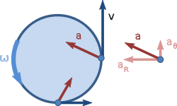
Figure 2: Velocity and acceleration for nonuniform circular motion: the velocity vector is tangential to the orbit, but the acceleration vector is not radially inward because of its tangential component a_θ that increases the rate of rotation: dω/dt = |a_θ|/R.

Particle trajectories in cylindrical-polar coordinates

See also: Generalized coordinates, Curvilinear coordinates, Orthogonal coordinates, and Frenet-Serret formulas

It is often convenient to formulate the trajectory of a particle r(t) = (x(t), y(t), z(t)) using polar coordinates in the X–Y plane. In this case, its velocity and acceleration take a convenient form.

Recall that the trajectory of a particle P is defined by its coordinate vector r measured in a fixed reference frame F. As the particle moves, its coordinate vector r(t) traces its trajectory, which is a curve in space, given by:

$${\displaystyle \mathbf {r} (t)=x(t){\hat {\mathbf {x} }}+y(t){\hat {\mathbf {y} }}+z(t){\hat {\mathbf {z} }},}$$

where x̂, ŷ, and ẑ are the unit vectors along the x, y and z axes of the reference frame F, respectively.

Consider a particle P that moves only on the surface of a circular cylinder r(t) = constant, it is possible to align the z axis of the fixed frame F with the axis of the cylinder. Then, the angle θ around this axis in the x–y plane can be used to define the trajectory as,

$${\displaystyle \mathbf {r} (t)=r\cos(\theta (t)){\hat {\mathbf {x} }}+r\sin(\theta (t)){\hat {\mathbf {y} }}+z(t){\hat {\mathbf {z} }},}$$

where the constant distance from the center is denoted as r, and θ(t) is a function of time.

The cylindrical coordinates for r(t) can be simplified by introducing the radial and tangential unit vectors,

$${\displaystyle {\hat {\mathbf {r} }}=\cos(\theta (t)){\hat {\mathbf {x} }}+\sin(\theta (t)){\hat {\mathbf {y} }},\quad {\hat {\mathbf {\theta } }}=-\sin(\theta (t)){\hat {\mathbf {x} }}+\cos(\theta (t)){\hat {\mathbf {y} }}.}$$

and their time derivatives from elementary calculus:

$${\displaystyle {\frac {{\text{d}}{\hat {\mathbf {r} }}}{{\text{d}}t}}=\omega {\hat {\mathbf {\theta } }}.}$$

$${\displaystyle {\frac {{\text{d}}^{2}{\hat {\mathbf {r} }}}{{\text{d}}t^{2}}}={\frac {{\text{d}}(\omega {\hat {\mathbf {\theta } }})}{{\text{d}}t}}=\alpha {\hat {\mathbf {\theta } }}-\omega {\hat {\mathbf {r} }}.}$$

$${\displaystyle {\frac {{\text{d}}{\hat {\mathbf {\theta } }}}{{\text{d}}t}}=-\theta {\hat {\mathbf {r} }}.}$$

$${\displaystyle {\frac {{\text{d}}^{2}{\hat {\mathbf {\theta } }}}{{\text{d}}t^{2}}}={\frac {{\text{d}}(-\theta {\hat {\mathbf {r} }})}{{\text{d}}t}}=-\alpha {\hat {\mathbf {r} }}-\omega ^{2}{\hat {\mathbf {\theta } }}.}$$

Using this notation, r(t) takes the form,

$${\displaystyle \mathbf {r} (t)=r{\hat {\mathbf {r} }}+z(t){\hat {\mathbf {z} }}.}$$

In general, the trajectory r(t) is not constrained to lie on a circular cylinder, so the radius R varies with time and the trajectory of the particle in cylindrical-polar coordinates becomes:

$${\displaystyle \mathbf {r} (t)=r(t){\hat {\mathbf {r} }}+z(t){\hat {\mathbf {z} }}.}$$

Where r, θ, and z might be continuously differentiable functions of time and the function notation is dropped for simplicity. The velocity vector v_P is the time derivative of the trajectory r(t), which yields:

$${\displaystyle \mathbf {v} _{P}={\frac {\text{d}}{{\text{d}}t}}\left(r{\hat {\mathbf {r} }}+z{\hat {\mathbf {z} }}\right)=v{\hat {\mathbf {r} }}+r\mathbf {\omega } {\hat {\mathbf {\theta } }}+v_{z}{\hat {\mathbf {z} }}=v({\hat {\mathbf {r} }}+{\hat {\mathbf {\theta } }})+v_{z}{\hat {\mathbf {z} }}.}$$

Similarly, the acceleration a_P, which is the time derivative of the velocity v_P, is given by:

$${\displaystyle \mathbf {a} _{P}={\frac {\text{d}}{{\text{d}}t}}\left(v{\hat {\mathbf {r} }}+v{\hat {\mathbf {\theta } }}+v_{z}{\hat {\mathbf {z} }}\right)=(a-v\theta ){\hat {\mathbf {r} }}+(a+v\omega ){\hat {\mathbf {\theta } }}+a_{z}{\hat {\mathbf {z} }}.}$$

The term ${\displaystyle -v\theta {\hat {\mathbf {r} }}}$ acts toward the center of curvature of the path at that point on the path, is commonly called the centripetal acceleration. The term ${\displaystyle v\omega {\hat {\mathbf {\theta } }}}$ is called the Coriolis acceleration.

Constant radius

If the trajectory of the particle is constrained to lie on a cylinder, then the radius r is constant and the velocity and acceleration vectors simplify. The velocity of v_P is the time derivative of the trajectory r(t),

$${\displaystyle \mathbf {v} _{P}={\frac {\text{d}}{{\text{d}}t}}\left(r{\hat {\mathbf {r} }}+z{\hat {\mathbf {z} }}\right)=r\omega {\hat {\mathbf {\theta } }}+v_{z}{\hat {\mathbf {z} }}=v{\hat {\mathbf {\theta } }}+v_{z}{\hat {\mathbf {z} }}.}$$

Planar circular trajectories

Each particle on the wheel travels in a planar circular trajectory (Kinematics of Machinery, 1876).

A special case of a particle trajectory on a circular cylinder occurs when there is no movement along the z axis:

$${\displaystyle \mathbf {r} (t)=r{\hat {\mathbf {r} }}+z{\hat {\mathbf {z} }},}$$

where r and z₀ are constants. In this case, the velocity v_P is given by:

$${\displaystyle \mathbf {v} _{P}={\frac {\text{d}}{{\text{d}}t}}\left(r{\hat {\mathbf {r} }}+z{\hat {\mathbf {z} }}\right)=r\omega {\hat {\mathbf {\theta } }}=v{\hat {\mathbf {\theta } }},}$$

where ${\displaystyle \omega }$ is the angular velocity of the unit vector θ^{^} around the z axis of the cylinder.

The acceleration a_P of the particle P is now given by:

$${\displaystyle \mathbf {a} _{P}={\frac {{\text{d}}(v{\hat {\mathbf {\theta } }})}{{\text{d}}t}}=a{\hat {\mathbf {\theta } }}-v\theta {\hat {\mathbf {r} }}.}$$

The components

$${\displaystyle a_{r}=-v\theta ,\quad a_{\theta }=a,}$$

are called, respectively, the radial and tangential components of acceleration.

The notation for angular velocity and angular acceleration is often defined as

$${\displaystyle \omega ={\dot {\theta }},\quad \alpha ={\ddot {\theta }},}$$

so the radial and tangential acceleration components for circular trajectories are also written as

$${\displaystyle a_{r}=-r\omega ^{2},\quad a_{\theta }=r\alpha .}$$

Point trajectories in a body moving in the plane

The movement of components of a mechanical system are analyzed by attaching a reference frame to each part and determining how the various reference frames move relative to each other. If the structural stiffness of the parts are sufficient, then their deformation can be neglected and rigid transformations can be used to define this relative movement. This reduces the description of the motion of the various parts of a complicated mechanical system to a problem of describing the geometry of each part and geometric association of each part relative to other parts.

Geometry is the study of the properties of figures that remain the same while the space is transformed in various ways—more technically, it is the study of invariants under a set of transformations. ^[19] These transformations can cause the displacement of the triangle in the plane, while leaving the vertex angle and the distances between vertices unchanged. Kinematics is often described as applied geometry, where the movement of a mechanical system is described using the rigid transformations of Euclidean geometry.

The coordinates of points in a plane are two-dimensional vectors in R² (two dimensional space). Rigid transformations are those that preserve the distance between any two points. The set of rigid transformations in an n-dimensional space is called the special Euclidean group on Rⁿ, and denoted SE(n).

Displacements and motion

The movement of each of the components of the Boulton & Watt Steam Engine (1784) is modeled by a continuous set of rigid displacements.

The position of one component of a mechanical system relative to another is defined by introducing a reference frame, say M, on one that moves relative to a fixed frame, F, on the other. The rigid transformation, or displacement, of M relative to F defines the relative position of the two components. A displacement consists of the combination of a rotation and a translation.

The set of all displacements of M relative to F is called the configuration space of M. A smooth curve from one position to another in this configuration space is a continuous set of displacements, called the motion of M relative to F. The motion of a body consists of a continuous set of rotations and translations.

Matrix representation

The combination of a rotation and translation in the plane R² can be represented by a certain type of 3×3 matrix known as a homogeneous transform. The 3×3 homogeneous transform is constructed from a 2×2 rotation matrix A(φ) and the 2×1 translation vector d = (d_x, d_y), as:

$${\displaystyle [T(\phi ,\mathbf {d} )]={\begin{bmatrix}A(\phi )&\mathbf {d} \\\mathbf {0} &1\end{bmatrix}}={\begin{bmatrix}\cos \phi &-\sin \phi &d_{x}\\\sin \phi &\cos \phi &d_{y}\\0&0&1\end{bmatrix}}.}$$

These homogeneous transforms perform rigid transformations on the points in the plane z = 1, that is, on points with coordinates r = (x, y, 1).

In particular, let r define the coordinates of points in a reference frame M coincident with a fixed frame F. Then, when the origin of M is displaced by the translation vector d relative to the origin of F and rotated by the angle φ relative to the x-axis of F, the new coordinates in F of points in M are given by:

$${\displaystyle \mathbf {P} =[T(\phi ,\mathbf {d} )]\mathbf {r} ={\begin{bmatrix}\cos \phi &-\sin \phi &d_{x}\\\sin \phi &\cos \phi &d_{y}\\0&0&1\end{bmatrix}}{\begin{bmatrix}x\\y\\1\end{bmatrix}}.}$$

Homogeneous transforms represent affine transformations. This formulation is necessary because a translation is not a linear transformation of R². However, using projective geometry, so that R² is considered a subset of R³, translations become affine linear transformations. ^[20]

Pure translation

If a rigid body moves so that its reference frame M does not rotate (θ = 0) relative to the fixed frame F, the motion is called pure translation. In this case, the trajectory of every point in the body is an offset of the trajectory d(t) of the origin of M, that is:

$${\displaystyle \mathbf {r} (t)=[T(0,\mathbf {d} (t))]\mathbf {p} =\mathbf {d} (t)+\mathbf {p} .}$$

Thus, for bodies in pure translation, the velocity and acceleration of every point P in the body are given by:

$${\displaystyle \mathbf {v} _{P}={\dot {\mathbf {r} }}(t)={\dot {\mathbf {d} }}(t)=\mathbf {v} _{O},\quad \mathbf {a} _{P}={\ddot {\mathbf {r} }}(t)={\ddot {\mathbf {d} }}(t)=\mathbf {a} _{O},}$$

where the dot denotes the derivative with respect to time and v_O and a_O are the velocity and acceleration, respectively, of the origin of the moving frame M. Recall the coordinate vector p in M is constant, so its derivative is zero.

Rotation of a body around a fixed axis

Main article: Rotation around a fixed axis

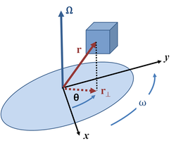
Figure 1: The angular velocity vector Ω points up for counterclockwise rotation and down for clockwise rotation, as specified by the right-hand rule. Angular position θ(t) changes with time at a rate ω(t) = dθ/dt.

Rotational or angular kinematics is the description of the rotation of an object. ^[21] In what follows, attention is restricted to simple rotation about an axis of fixed orientation. The z-axis has been chosen for convenience.

Position

This allows the description of a rotation as the angular position of a planar reference frame M relative to a fixed F about this shared z-axis. Coordinates p = (x, y) in M are related to coordinates P = (X, Y) in F by the matrix equation:

$${\displaystyle \mathbf {P} (t)=[A(t)]\mathbf {p} ,}$$

where

$${\displaystyle [A(t)]={\begin{bmatrix}\cos(\theta (t))&-\sin(\theta (t))\\\sin(\theta (t))&\cos(\theta (t))\end{bmatrix}},}$$

is the rotation matrix that defines the angular position of M relative to F as a function of time.

Velocity

If the point p does not move in M, its velocity in F is given by

$${\displaystyle \mathbf {v} _{P}={\dot {\mathbf {P} }}=[{\dot {A}}(t)]\mathbf {p} .}$$

It is convenient to eliminate the coordinates p and write this as an operation on the trajectory P(t),

$${\displaystyle \mathbf {v} _{P}=[{\dot {A}}(t)][A(t)^{-1}]\mathbf {P} =[\Omega ]\mathbf {P} ,}$$

where the matrix

$${\displaystyle [\Omega ]={\begin{bmatrix}0&-\omega \\\omega &0\end{bmatrix}},}$$

is known as the angular velocity matrix of M relative to F. The parameter ω is the time derivative of the angle θ, that is:

$${\displaystyle \omega ={\frac {{\text{d}}\theta }{{\text{d}}t}}.}$$

Acceleration

The acceleration of P(t) in F is obtained as the time derivative of the velocity,

$${\displaystyle \mathbf {A} _{P}={\ddot {P}}(t)=[{\dot {\Omega }}]\mathbf {P} +[\Omega ]{\dot {\mathbf {P} }},}$$

which becomes

$${\displaystyle \mathbf {A} _{P}=[{\dot {\Omega }}]\mathbf {P} +[\Omega ][\Omega ]\mathbf {P} ,}$$

where

$${\displaystyle [{\dot {\Omega }}]={\begin{bmatrix}0&-\alpha \\\alpha &0\end{bmatrix}},}$$

is the angular acceleration matrix of M on F, and

$${\displaystyle \alpha ={\frac {{\text{d}}^{2}\theta }{{\text{d}}t^{2}}}.}$$

The description of rotation then involves these three quantities:

• Angular position: the oriented distance from a selected origin on the rotational axis to a point of an object is a vector r(t) locating the point. The vector r(t) has some projection (or, equivalently, some component) r_⊥(t) on a plane perpendicular to the axis of rotation. Then the angular position of that point is the angle θ from a reference axis (typically the positive x-axis) to the vector r_⊥(t) in a known rotation sense (typically given by the right-hand rule).
• Angular velocity: the angular velocity ω is the rate at which the angular position θ changes with respect to time t:
  $${\displaystyle \omega ={\frac {{\text{d}}\theta }{{\text{d}}t}}}$$
  The angular velocity is represented in Figure 1 by a vector Ω pointing along the axis of rotation with magnitude ω and sense determined by the direction of rotation as given by the right-hand rule.
• Angular acceleration: the magnitude of the angular acceleration α is the rate at which the angular velocity ω changes with respect to time t:
  $${\displaystyle \alpha ={\frac {{\text{d}}\omega }{{\text{d}}t}}}$$

The equations of translational kinematics can easily be extended to planar rotational kinematics for constant angular acceleration with simple variable exchanges:

$${\displaystyle \omega _{\mathrm {f} }=\omega _{\mathrm {i} }+\alpha t\!}$$

$${\displaystyle \theta _{\mathrm {f} }-\theta _{\mathrm {i} }=\omega _{\mathrm {i} }t+{\tfrac {1}{2}}\alpha t^{2}}$$

$${\displaystyle \theta _{\mathrm {f} }-\theta _{\mathrm {i} }={\tfrac {1}{2}}(\omega _{\mathrm {f} }+\omega _{\mathrm {i} })t}$$

$${\displaystyle \omega _{\mathrm {f} }^{2}=\omega _{\mathrm {i} }^{2}+2\alpha (\theta _{\mathrm {f} }-\theta _{\mathrm {i} }).}$$

Here θ_i and θ_f are, respectively, the initial and final angular positions, ω_i and ω_f are, respectively, the initial and final angular velocities, and α is the constant angular acceleration. Although position in space and velocity in space are both true vectors (in terms of their properties under rotation), as is angular velocity, angle itself is not a true vector.

Point trajectories in body moving in three dimensions

Important formulas in kinematics define the velocity and acceleration of points in a moving body as they trace trajectories in three-dimensional space. This is particularly important for the center of mass of a body, which is used to derive equations of motion using either Newton's second law or Lagrange's equations.

Position

In order to define these formulas, the movement of a component B of a mechanical system is defined by the set of rotations [A(t)] and translations d(t) assembled into the homogeneous transformation [T(t)]=[A(t), d(t)]. If p is the coordinates of a point P in B measured in the moving reference frame M, then the trajectory of this point traced in F is given by:

$${\displaystyle \mathbf {P} (t)=[T(t)]\mathbf {p} ={\begin{bmatrix}\mathbf {P} \\1\end{bmatrix}}={\begin{bmatrix}A(t)&\mathbf {d} (t)\\0&1\end{bmatrix}}{\begin{bmatrix}\mathbf {p} \\1\end{bmatrix}}.}$$

This notation does not distinguish between P = (X, Y, Z, 1), and P = (X, Y, Z), which is hopefully clear in context.

This equation for the trajectory of P can be inverted to compute the coordinate vector p in M as:

$${\displaystyle \mathbf {p} =[T(t)]^{-1}\mathbf {P} (t)={\begin{bmatrix}\mathbf {p} \\1\end{bmatrix}}={\begin{bmatrix}A(t)^{\text{T}}&-A(t)^{\text{T}}\mathbf {d} (t)\\0&1\end{bmatrix}}{\begin{bmatrix}\mathbf {P} (t)\\1\end{bmatrix}}.}$$

This expression uses the fact that the transpose of a rotation matrix is also its inverse, that is:

$${\displaystyle [A(t)]^{\text{T}}[A(t)]=I.\!}$$

Velocity

The velocity of the point P along its trajectory P(t) is obtained as the time derivative of this position vector,

$${\displaystyle \mathbf {v} _{P}=[{\dot {T}}(t)]\mathbf {p} ={\begin{bmatrix}\mathbf {v} _{P}\\0\end{bmatrix}}=\left({\frac {d}{dt}}{\begin{bmatrix}A(t)&\mathbf {d} (t)\\0&1\end{bmatrix}}\right){\begin{bmatrix}\mathbf {p} \\1\end{bmatrix}}={\begin{bmatrix}{\dot {A}}(t)&{\dot {\mathbf {d} }}(t)\\0&0\end{bmatrix}}{\begin{bmatrix}\mathbf {p} \\1\end{bmatrix}}.}$$

The dot denotes the derivative with respect to time; because p is constant, its derivative is zero.

This formula can be modified to obtain the velocity of P by operating on its trajectory P(t) measured in the fixed frame F. Substituting the inverse transform for p into the velocity equation yields:

$${\displaystyle {\begin{aligned}\mathbf {v} _{P}&=[{\dot {T}}(t)][T(t)]^{-1}\mathbf {P} (t)\\[4pt]&={\begin{bmatrix}\mathbf {v} _{P}\\0\end{bmatrix}}={\begin{bmatrix}{\dot {A}}&{\dot {\mathbf {d} }}\\0&0\end{bmatrix}}{\begin{bmatrix}A&\mathbf {d} \\0&1\end{bmatrix}}^{-1}{\begin{bmatrix}\mathbf {P} (t)\\1\end{bmatrix}}\\[4pt]&={\begin{bmatrix}{\dot {A}}&{\dot {\mathbf {d} }}\\0&0\end{bmatrix}}A^{-1}{\begin{bmatrix}1&-\mathbf {d} \\0&A\end{bmatrix}}{\begin{bmatrix}\mathbf {P} (t)\\1\end{bmatrix}}\\[4pt]&={\begin{bmatrix}{\dot {A}}A^{-1}&-{\dot {A}}A^{-1}\mathbf {d} +{\dot {\mathbf {d} }}\\0&0\end{bmatrix}}{\begin{bmatrix}\mathbf {P} (t)\\1\end{bmatrix}}\\[4pt]&={\begin{bmatrix}{\dot {A}}A^{\text{T}}&-{\dot {A}}A^{\text{T}}\mathbf {d} +{\dot {\mathbf {d} }}\\0&0\end{bmatrix}}{\begin{bmatrix}\mathbf {P} (t)\\1\end{bmatrix}}\\[6pt]\mathbf {v} _{P}&=[S]\mathbf {P} .\end{aligned}}}$$

The matrix [S] is given by:

$${\displaystyle [S]={\begin{bmatrix}\Omega &-\Omega \mathbf {d} +{\dot {\mathbf {d} }}\\0&0\end{bmatrix}}}$$

where

$${\displaystyle [\Omega ]={\dot {A}}A^{\text{T}},}$$

is the angular velocity matrix.

Multiplying by the operator [S], the formula for the velocity v_P takes the form:

$${\displaystyle \mathbf {v} _{P}=[\Omega ](\mathbf {P} -\mathbf {d} )+{\dot {\mathbf {d} }}=\omega \times \mathbf {R} _{P/O}+\mathbf {v} _{O},}$$

where the vector ω is the angular velocity vector obtained from the components of the matrix [Ω]; the vector

$${\displaystyle \mathbf {R} _{P/O}=\mathbf {P} -\mathbf {d} ,}$$

is the position of P relative to the origin O of the moving frame M; and

$${\displaystyle \mathbf {v} _{O}={\dot {\mathbf {d} }},}$$

is the velocity of the origin O.

Acceleration

The acceleration of a point P in a moving body B is obtained as the time derivative of its velocity vector:

$${\displaystyle \mathbf {A} _{P}={\frac {d}{dt}}\mathbf {v} _{P}={\frac {d}{dt}}\left([S]\mathbf {P} \right)=[{\dot {S}}]\mathbf {P} +[S]{\dot {\mathbf {P} }}=[{\dot {S}}]\mathbf {P} +[S][S]\mathbf {P} .}$$

This equation can be expanded firstly by computing

$${\displaystyle [{\dot {S}}]={\begin{bmatrix}{\dot {\Omega }}&-{\dot {\Omega }}\mathbf {d} -\Omega {\dot {\mathbf {d} }}+{\ddot {\mathbf {d} }}\\0&0\end{bmatrix}}={\begin{bmatrix}{\dot {\Omega }}&-{\dot {\Omega }}\mathbf {d} -\Omega \mathbf {v} _{O}+\mathbf {A} _{O}\\0&0\end{bmatrix}}}$$

and

$${\displaystyle [S]^{2}={\begin{bmatrix}\Omega &-\Omega \mathbf {d} +\mathbf {v} _{O}\\0&0\end{bmatrix}}^{2}={\begin{bmatrix}\Omega ^{2}&-\Omega ^{2}\mathbf {d} +\Omega \mathbf {v} _{O}\\0&0\end{bmatrix}}.}$$

The formula for the acceleration A_P can now be obtained as:

$${\displaystyle \mathbf {A} _{P}={\dot {\Omega }}(\mathbf {P} -\mathbf {d} )+\mathbf {A} _{O}+\Omega ^{2}(\mathbf {P} -\mathbf {d} ),}$$

or

$${\displaystyle \mathbf {A} _{P}=\alpha \times \mathbf {R} _{P/O}+\omega \times \omega \times \mathbf {R} _{P/O}+\mathbf {A} _{O},}$$

where α is the angular acceleration vector obtained from the derivative of the angular velocity matrix;

$${\displaystyle \mathbf {R} _{P/O}=\mathbf {P} -\mathbf {d} ,}$$

is the relative position vector (the position of P relative to the origin O of the moving frame M); and

$${\displaystyle \mathbf {A} _{O}={\ddot {\mathbf {d} }}}$$

is the acceleration of the origin of the moving frame M.

Kinematic constraints

Kinematic constraints are constraints on the movement of components of a mechanical system. Kinematic constraints can be considered to have two basic forms, (i) constraints that arise from hinges, sliders and cam joints that define the construction of the system, called holonomic constraints, and (ii) constraints imposed on the velocity of the system such as the knife-edge constraint of ice-skates on a flat plane, or rolling without slipping of a disc or sphere in contact with a plane, which are called non-holonomic constraints. The following are some common examples.

Kinematic coupling

A kinematic coupling exactly constrains all 6 degrees of freedom.

Rolling without slipping

An object that rolls against a surface without slipping obeys the condition that the velocity of its center of mass is equal to the cross product of its angular velocity with a vector from the point of contact to the center of mass:

$${\displaystyle {\boldsymbol {v}}_{G}(t)={\boldsymbol {\Omega }}\times {\boldsymbol {r}}_{G/O}.}$$

For the case of an object that does not tip or turn, this reduces to ${\displaystyle v=r\omega }$.

Inextensible cord

This is the case where bodies are connected by an idealized cord that remains in tension and cannot change length. The constraint is that the sum of lengths of all segments of the cord is the total length, and accordingly the time derivative of this sum is zero. ^{[22] [23] [24]} A dynamic problem of this type is the pendulum. Another example is a drum turned by the pull of gravity upon a falling weight attached to the rim by the inextensible cord. ^[25] An equilibrium problem (i.e. not kinematic) of this type is the catenary. ^[26]

Kinematic pairs

Main article: Kinematic pair

Reuleaux called the ideal connections between components that form a machine kinematic pairs. He distinguished between higher pairs which were said to have line contact between the two links and lower pairs that have area contact between the links. J. Phillips shows that there are many ways to construct pairs that do not fit this simple classification. ^[27]

Lower pair

A lower pair is an ideal joint, or holonomic constraint, that maintains contact between a point, line or plane in a moving solid (three-dimensional) body to a corresponding point line or plane in the fixed solid body. There are the following cases:

• A revolute pair, or hinged joint, requires a line, or axis, in the moving body to remain co-linear with a line in the fixed body, and a plane perpendicular to this line in the moving body maintain contact with a similar perpendicular plane in the fixed body. This imposes five constraints on the relative movement of the links, which therefore has one degree of freedom, which is pure rotation about the axis of the hinge.
• A prismatic joint, or slider, requires that a line, or axis, in the moving body remain co-linear with a line in the fixed body, and a plane parallel to this line in the moving body maintain contact with a similar parallel plane in the fixed body. This imposes five constraints on the relative movement of the links, which therefore has one degree of freedom. This degree of freedom is the distance of the slide along the line.
• A cylindrical joint requires that a line, or axis, in the moving body remain co-linear with a line in the fixed body. It is a combination of a revolute joint and a sliding joint. This joint has two degrees of freedom. The position of the moving body is defined by both the rotation about and slide along the axis.
• A spherical joint, or ball joint, requires that a point in the moving body maintain contact with a point in the fixed body. This joint has three degrees of freedom.
• A planar joint requires that a plane in the moving body maintain contact with a plane in fixed body. This joint has three degrees of freedom.

Higher pairs

Generally speaking, a higher pair is a constraint that requires a curve or surface in the moving body to maintain contact with a curve or surface in the fixed body. For example, the contact between a cam and its follower is a higher pair called a cam joint. Similarly, the contact between the involute curves that form the meshing teeth of two gears are cam joints.

Kinematic chains

Illustration of a four-bar linkage from Kinematics of Machinery, 1876

Rigid bodies ("links") connected by kinematic pairs ("joints") are known as kinematic chains . Mechanisms and robots are examples of kinematic chains. The degree of freedom of a kinematic chain is computed from the number of links and the number and type of joints using the mobility formula. This formula can also be used to enumerate the topologies of kinematic chains that have a given degree of freedom, which is known as type synthesis in machine design.

Examples

The planar one degree-of-freedom linkages assembled from N links and j hinges or sliding joints are:

• N = 2, j = 1 : a two-bar linkage that is the lever;
• N = 4, j = 4 : the four-bar linkage;
• N = 6, j = 7 : a six-bar linkage. This must have two links ("ternary links") that support three joints. There are two distinct topologies that depend on how the two ternary linkages are connected. In the Watt topology, the two ternary links have a common joint; in the Stephenson topology, the two ternary links do not have a common joint and are connected by binary links. ^[28]
• N = 8, j = 10 : eight-bar linkage with 16 different topologies;
• N = 10, j = 13 : ten-bar linkage with 230 different topologies;
• N = 12, j = 16 : twelve-bar linkage with 6,856 topologies.

For larger chains and their linkage topologies, see R. P. Sunkari and L. C. Schmidt, "Structural synthesis of planar kinematic chains by adapting a Mckay-type algorithm", Mechanism and Machine Theory #41, pp. 1021–1030 (2006).

See also

• Absement
• Acceleration
• Affine geometry § Kinematics
• Analytical mechanics
• Applied mechanics
• Celestial mechanics
• Centripetal force
• Classical mechanics
• Distance
• Dynamics (physics)
• Fictitious force
• Forward kinematics
• Four-bar linkage
• Inverse kinematics
• Jerk (physics)
• Kepler's laws
• Kinematic coupling
• Kinematic diagram
• Kinematic synthesis
• Kinetics (physics)
• Motion (physics)
• Orbital mechanics
• Statics
• Velocity
• Integral kinematics
• Chebychev–Grübler–Kutzbach criterion

References

1. Edmund Taylor Whittaker (1904). A Treatise on the Analytical Dynamics of Particles and Rigid Bodies . Cambridge University Press. Chapter 1. ISBN   0-521-35883-3.
2. Joseph Stiles Beggs (1983). Kinematics. Taylor & Francis. p. 1. ISBN   0-89116-355-7.
3. Thomas Wallace Wright (1896). Elements of Mechanics Including Kinematics, Kinetics and Statics. E and FN Spon. Chapter 1.
4. Russell C. Hibbeler (2009). "Kinematics and kinetics of a particle". Engineering Mechanics: Dynamics (12th ed.). Prentice Hall. p. 298. ISBN   978-0-13-607791-6.
5. Ahmed A. Shabana (2003). "Reference kinematics". Dynamics of Multibody Systems (2nd ed.). Cambridge University Press. ISBN   978-0-521-54411-5.
6. P. P. Teodorescu (2007). "Kinematics". Mechanical Systems, Classical Models: Particle Mechanics. Springer. p. 287. ISBN   978-1-4020-5441-9..
7. A. Biewener (2003). Animal Locomotion. Oxford University Press. ISBN   019850022X.
8. J. M. McCarthy and G. S. Soh, 2010, Geometric Design of Linkages, Springer, New York.
9. Ampère, André-Marie (1834). Essai sur la Philosophie des Sciences. Chez Bachelier.
10. Merz, John (1903). A History of European Thought in the Nineteenth Century. Blackwood, London. pp.  5.
11. O. Bottema & B. Roth (1990). Theoretical Kinematics. Dover Publications. preface, p. 5. ISBN   0-486-66346-9.
12. Harper, Douglas. "cinema". Online Etymology Dictionary .
13. Crash course physics
14. 2.4 Integration, MIT, archived from the original on 2021-11-13, retrieved 2021-07-04
15. https://www.youtube.com/watch?v=jLJLXka2wEM Crash course physics integrals
16. https://www.mathsisfun.com/algebra/trig-area-triangle-without-right-angle.html Area of Triangles Without Right Angles
17. kinematics.gif (508×368) (Image). Retrieved 3 November 2023.
18. Reuleaux, F.; Kennedy, Alex B. W. (1876), The Kinematics of Machinery: Outlines of a Theory of Machines, London: Macmillan
19. Geometry: the study of properties of given elements that remain invariant under specified transformations. "Definition of geometry". Merriam-Webster on-line dictionary. 31 May 2023.
20. Paul, Richard (1981). Robot manipulators: mathematics, programming, and control : the computer control of robot manipulators. MIT Press, Cambridge, MA. ISBN   978-0-262-16082-7.
21. R. Douglas Gregory (2006). Chapter 16. Cambridge, England: Cambridge University. ISBN   0-521-82678-0.
22. William Thomson Kelvin & Peter Guthrie Tait (1894). Elements of Natural Philosophy. Cambridge University Press. p.  4. ISBN   1-57392-984-0.
23. William Thomson Kelvin & Peter Guthrie Tait (1894). Elements of Natural Philosophy. p. 296.
24. M. Fogiel (1980). "Problem 17-11". The Mechanics Problem Solver. Research & Education Association. p. 613. ISBN   0-87891-519-2.
25. Irving Porter Church (1908). Mechanics of Engineering. Wiley. p.  111. ISBN   1-110-36527-6.
26. Morris Kline (1990). Mathematical Thought from Ancient to Modern Times . Oxford University Press. p.  472. ISBN   0-19-506136-5.
27. Phillips, Jack (2007). Freedom in Machinery, Volumes 1–2 (reprint ed.). Cambridge University Press. ISBN   978-0-521-67331-0.
28. Tsai, Lung-Wen (2001). Mechanism design:enumeration of kinematic structures according to function (illustrated ed.). CRC Press. p. 121. ISBN   978-0-8493-0901-4.

1. While τ is used as the variable of integration, some authors may use t′ as the variable of integration, although that can be confused with Lagrange's notation for derivatives ^[14]

Further reading

• Koetsier, Teun (1994), "§8.3 Kinematics", in Grattan-Guinness, Ivor (ed.), Companion Encyclopedia of the History and Philosophy of the Mathematical Sciences, vol. 2, Routledge, pp. 994–1001, ISBN   0-415-09239-6
• Moon, Francis C. (2007). The Machines of Leonardo Da Vinci and Franz Reuleaux, Kinematics of Machines from the Renaissance to the 20th Century. Springer. ISBN   978-1-4020-5598-0.
• Eduard Study (1913) D.H. Delphenich translator, "Foundations and goals of analytical kinematics".

External links

• Java applet of 1D kinematics
• Physclips: Mechanics with animations and video clips from the University of New South Wales.
• Kinematic Models for Design Digital Library (KMODDL), featuring movies and photos of hundreds of working models of mechanical systems at Cornell University and an e-book library of classic texts on mechanical design and engineering.
• Micro-Inch Positioning with Kinematic Components