
In physics, the Navier–Stokes equations are partial differential equations which describe the motion of viscous fluid substances, named after French engineer and physicist Claude-Louis Navier and Anglo-Irish physicist and mathematician George Gabriel Stokes. They were developed over several decades of progressively building the theories, from 1822 (Navier) to 1842-1850 (Stokes).
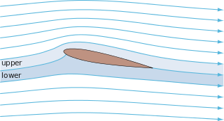
In fluid dynamics, potential flow describes the velocity field as the gradient of a scalar function: the velocity potential. As a result, a potential flow is characterized by an irrotational velocity field, which is a valid approximation for several applications. The irrotationality of a potential flow is due to the curl of the gradient of a scalar always being equal to zero.
The vorticity equation of fluid dynamics describes the evolution of the vorticity ω of a particle of a fluid as it moves with its flow; that is, the local rotation of the fluid. The governing equation is:
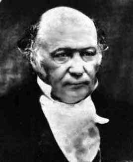
Hamiltonian mechanics emerged in 1833 as a reformulation of Lagrangian mechanics. Introduced by Sir William Rowan Hamilton, Hamiltonian mechanics replaces (generalized) velocities used in Lagrangian mechanics with (generalized) momenta. Both theories provide interpretations of classical mechanics and describe the same physical phenomena.
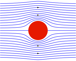
In 1851, George Gabriel Stokes derived an expression, now known as Stokes' law, for the frictional force – also called drag force – exerted on spherical objects with very small Reynolds numbers in a viscous fluid. Stokes' law is derived by solving the Stokes flow limit for small Reynolds numbers of the Navier–Stokes equations.
The stream function is defined for incompressible (divergence-free) flows in two dimensions – as well as in three dimensions with axisymmetry. The flow velocity components can be expressed as the derivatives of the scalar stream function. The stream function can be used to plot streamlines, which represent the trajectories of particles in a steady flow. The two-dimensional Lagrange stream function was introduced by Joseph Louis Lagrange in 1781. The Stokes stream function is for axisymmetrical three-dimensional flow, and is named after George Gabriel Stokes.
Rossby waves, also known as planetary waves, are a type of inertial wave naturally occurring in rotating fluids. They were first identified by Sweden-born American meteorologist Carl-Gustaf Arvid Rossby. They are observed in the atmospheres and oceans of Earth and other planets, owing to the rotation of Earth or of the planet involved. Atmospheric Rossby waves on Earth are giant meanders in high-altitude winds that have a major influence on weather. These waves are associated with pressure systems and the jet stream. Oceanic Rossby waves move along the thermocline: the boundary between the warm upper layer and the cold deeper part of the ocean.
One of the guiding principles in modern chemical dynamics and spectroscopy is that the motion of the nuclei in a molecule is slow compared to that of its electrons. This is justified by the large disparity between the mass of an electron and the typical mass of a nucleus and leads to the Born–Oppenheimer approximation and the idea that the structure and dynamics of a chemical species are largely determined by nuclear motion on potential energy surfaces. The potential energy surfaces are obtained within the adiabatic or Born–Oppenheimer approximation. This corresponds to a representation of the molecular wave function where the variables corresponding to the molecular geometry and the electronic degrees of freedom are separated. The non separable terms are due to the nuclear kinetic energy terms in the molecular Hamiltonian and are said to couple the potential energy surfaces. In the neighbourhood of an avoided crossing or conical intersection, these terms cannot be neglected. One therefore usually performs one unitary transformation from the adiabatic representation to the so-called diabatic representation in which the nuclear kinetic energy operator is diagonal. In this representation, the coupling is due to the electronic energy and is a scalar quantity that is significantly easier to estimate numerically.
Hamiltonian fluid mechanics is the application of Hamiltonian methods to fluid mechanics. Note that this formalism only applies to nondissipative fluids.
In fluid mechanics, potential vorticity (PV) is a quantity which is proportional to the dot product of vorticity and stratification. This quantity, following a parcel of air or water, can only be changed by diabatic or frictional processes. It is a useful concept for understanding the generation of vorticity in cyclogenesis, especially along the polar front, and in analyzing flow in the ocean.
In quantum mechanics, the Pauli equation or Schrödinger–Pauli equation is the formulation of the Schrödinger equation for spin-½ particles, which takes into account the interaction of the particle's spin with an external electromagnetic field. It is the non-relativistic limit of the Dirac equation and can be used where particles are moving at speeds much less than the speed of light, so that relativistic effects can be neglected. It was formulated by Wolfgang Pauli in 1927.
The intent of this article is to highlight the important points of the derivation of the Navier–Stokes equations as well as its application and formulation for different families of fluids.

In fluid dynamics, the Stokes stream function is used to describe the streamlines and flow velocity in a three-dimensional incompressible flow with axisymmetry. A surface with a constant value of the Stokes stream function encloses a streamtube, everywhere tangential to the flow velocity vectors. Further, the volume flux within this streamtube is constant, and all the streamlines of the flow are located on this surface. The velocity field associated with the Stokes stream function is solenoidal—it has zero divergence. This stream function is named in honor of George Gabriel Stokes.
In fluid dynamics, Luke's variational principle is a Lagrangian variational description of the motion of surface waves on a fluid with a free surface, under the action of gravity. This principle is named after J.C. Luke, who published it in 1967. This variational principle is for incompressible and inviscid potential flows, and is used to derive approximate wave models like the mild-slope equation, or using the averaged Lagrangian approach for wave propagation in inhomogeneous media.
In fluid dynamics, the Oseen equations describe the flow of a viscous and incompressible fluid at small Reynolds numbers, as formulated by Carl Wilhelm Oseen in 1910. Oseen flow is an improved description of these flows, as compared to Stokes flow, with the (partial) inclusion of convective acceleration.

In fluid dynamics, the mild-slope equation describes the combined effects of diffraction and refraction for water waves propagating over bathymetry and due to lateral boundaries—like breakwaters and coastlines. It is an approximate model, deriving its name from being originally developed for wave propagation over mild slopes of the sea floor. The mild-slope equation is often used in coastal engineering to compute the wave-field changes near harbours and coasts.
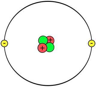
A helium atom is an atom of the chemical element helium. Helium is composed of two electrons bound by the electromagnetic force to a nucleus containing two protons along with either one or two neutrons, depending on the isotope, held together by the strong force. Unlike for hydrogen, a closed-form solution to the Schrödinger equation for the helium atom has not been found. However, various approximations, such as the Hartree–Fock method, can be used to estimate the ground state energy and wavefunction of the atom.

In continuum mechanics, Whitham's averaged Lagrangian method – or in short Whitham's method – is used to study the Lagrangian dynamics of slowly-varying wave trains in an inhomogeneous (moving) medium. The method is applicable to both linear and non-linear systems. As a direct consequence of the averaging used in the method, wave action is a conserved property of the wave motion. In contrast, the wave energy is not necessarily conserved, due to the exchange of energy with the mean motion. However the total energy, the sum of the energies in the wave motion and the mean motion, will be conserved for a time-invariant Lagrangian. Further, the averaged Lagrangian has a strong relation to the dispersion relation of the system.
In fluid dynamics, the Craik–Leibovich (CL) vortex force describes a forcing of the mean flow through wave–current interaction, specifically between the Stokes drift velocity and the mean-flow vorticity. The CL vortex force is used to explain the generation of Langmuir circulations by an instability mechanism. The CL vortex-force mechanism was derived and studied by Sidney Leibovich and Alex D. D. Craik in the 1970s and 80s, in their studies of Langmuir circulations.
In fluid dynamics, Beltrami flows are flows in which the vorticity vector and the velocity vector are parallel to each other. In other words, Beltrami flow is a flow where Lamb vector is zero. It is named after the Italian mathematician Eugenio Beltrami due to his derivation of the Beltrami vector field, while initial developments in fluid dynamics were done by the Russian scientist Ippolit S. Gromeka in 1881.


