Fick's laws of diffusion

For the technique of measuring cardiac output, see Fick principle.

Molecular diffusion from a microscopic and macroscopic point of view. Initially, there are solute molecules on the left side of a barrier (purple line) and none on the right. The barrier is removed, and the solute diffuses to fill the whole container. Top: A single molecule moves around randomly. Middle: With more molecules, there is a clear trend where the solute fills the container more and more uniformly. Bottom: With an enormous number of solute molecules, randomness becomes undetectable: The solute appears to move smoothly and systematically from high-concentration areas to low-concentration areas. This smooth flow is described by Fick's laws.

Fick's laws of diffusion describe diffusion and were first posited by Adolf Fick in 1855 on the basis of largely experimental results. They can be used to solve for the diffusion coefficient, D. Fick's first law can be used to derive his second law which in turn is identical to the diffusion equation.

Fick's first law: Movement of particles from high to low concentration (diffusive flux) is directly proportional to the particle's concentration gradient. ^[1]

Fick's second law: Prediction of change in concentration gradient with time due to diffusion.

A diffusion process that obeys Fick's laws is called normal or Fickian diffusion; otherwise, it is called anomalous diffusion or non-Fickian diffusion.

History

In 1855, physiologist Adolf Fick first reported ^[2] his now well-known laws governing the transport of mass through diffusive means. Fick's work was inspired by the earlier experiments of Thomas Graham, which fell short of proposing the fundamental laws for which Fick would become famous. Fick's law is analogous to the relationships discovered at the same epoch by other eminent scientists: Darcy's law (hydraulic flow), Ohm's law (charge transport), and Fourier's Law (heat transport).

Fick's experiments (modeled on Graham's) dealt with measuring the concentrations and fluxes of salt, diffusing between two reservoirs through tubes of water. It is notable that Fick's work primarily concerned diffusion in fluids, because at the time, diffusion in solids was not considered generally possible. ^[3] Today, Fick's Laws form the core of our understanding of diffusion in solids, liquids, and gases (in the absence of bulk fluid motion in the latter two cases). When a diffusion process does not follow Fick's laws (which happens in cases of diffusion through porous media and diffusion of swelling penetrants, among others), ^{[4] [5]} it is referred to as non-Fickian.

Fick's first law

Fick's first law relates the diffusive flux to the gradient of the concentration. It postulates that the flux goes from regions of high concentration to regions of low concentration, with a magnitude that is proportional to the concentration gradient (spatial derivative), or in simplistic terms the concept that a solute will move from a region of high concentration to a region of low concentration across a concentration gradient. In one (spatial) dimension, the law can be written in various forms, where the most common form (see ^{[6] [7]} ) is in a molar basis:

${\displaystyle J=-D{\frac {d\varphi }{dx}}}$

where

• J is the diffusion flux, of which the dimension is the amount of substance per unit area per unit time. J measures the amount of substance that will flow through a unit area during a unit time interval.
• D is the diffusion coefficient or diffusivity . Its dimension is area per unit time.
• ${\displaystyle {\frac {d\varphi }{dx}}}$ is the concentration gradient
• φ (for ideal mixtures) is the concentration, with a dimension of amount of substance per unit volume.
• x is position, the dimension of which is length.

D is proportional to the squared velocity of the diffusing particles, which depends on the temperature, viscosity of the fluid and the size of the particles according to the Stokes–Einstein relation. In dilute aqueous solutions the diffusion coefficients of most ions are similar and have values that at room temperature are in the range of (0.6–2)×10⁻⁹ m²/s. For biological molecules the diffusion coefficients normally range from 10⁻¹⁰ to 10⁻¹¹ m²/s.

In two or more dimensions we must use ∇, the del or gradient operator, which generalises the first derivative, obtaining

${\displaystyle \mathbf {J} =-D\nabla \varphi }$

where J denotes the diffusion flux vector.

The driving force for the one-dimensional diffusion is the quantity −∂φ/∂x, which for ideal mixtures is the concentration gradient.

Variations of the first law

Another form for the first law is to write it with the primary variable as mass fraction (y_i, given for example in kg/kg), then the equation changes to:

${\displaystyle \mathbf {J} _{i}=-{\frac {\rho D}{M_{i}}}\nabla y_{i}}$

where

• the index i denotes the ith species,
• J_i is the diffusion flux vector of the ith species (for example in mol/m²-s),
• M_i is the molar mass of the ith species, and
• ρ is the mixture density (for example in kg/m³).

The ${\displaystyle \rho }$ is outside the gradient operator. This is because:

${\displaystyle y_{i}={\frac {\rho _{si}}{\rho }}}$

where ρ_si is the partial density of the ith species.

Beyond this, in chemical systems other than ideal solutions or mixtures, the driving force for diffusion of each species is the gradient of chemical potential of this species. Then Fick's first law (one-dimensional case) can be written

${\displaystyle J_{i}=-{\frac {Dc_{i}}{RT}}{\frac {\partial \mu _{i}}{\partial x}}}$

where

• the index i denotes the ith species
• c is the concentration (mol/m³)
• R is the universal gas constant (J/K/mol)
• T is the absolute temperature (K)
• μ is the chemical potential (J/mol).

The driving force of Fick's law can be expressed as a fugacity difference:

${\displaystyle J_{i}=-{\frac {D}{RT}}{\frac {\partial f_{i}}{\partial x}}}$

Fugacity ${\displaystyle f_{i}}$ has Pa units. ${\displaystyle f_{i}}$ is a partial pressure of component i in a vapor ${\displaystyle f_{i}^{\text{G}}}$ or liquid ${\displaystyle f_{i}^{\text{L}}}$ phase. At vapor liquid equilibrium the evaporation flux is zero because ${\displaystyle f_{i}^{\text{G}}=f_{i}^{\text{L}}}$.

Derivation of Fick's first law for gases

Four versions of Fick's law for binary gas mixtures are given below. These assume: thermal diffusion is negligible; the body force per unit mass is the same on both species; and either pressure is constant or both species have the same molar mass. Under these conditions, Ref. ^[8] shows in detail how the diffusion equation from the kinetic theory of gases reduces to this version of Fick's law:

$${\displaystyle \mathbf {V_{i}} =-D\nabla \ln y_{i},}$$

where V_i is the diffusion velocity of species i. In terms of species flux this is

$${\displaystyle \mathbf {J_{i}} =-{\frac {\rho D}{M_{i}}}\nabla y_{i}.}$$

If, additionally, ${\displaystyle \nabla \rho =0}$, this reduces to the most common form of Fick's law,

$${\displaystyle \mathbf {J_{i}} =-D\nabla \varphi .}$$

If (instead of or in addition to ${\displaystyle \nabla \rho =0}$) both species have the same molar mass, Fick's law becomes

$${\displaystyle \mathbf {J_{i}} =-{\frac {\rho D}{M_{i}}}\nabla x_{i},}$$

where ${\displaystyle x_{i}}$ is the mole fraction of species i.

Fick's second law

Fick's second law predicts how diffusion causes the concentration to change with respect to time. It is a partial differential equation which in one dimension reads:

${\displaystyle {\frac {\partial \varphi }{\partial t}}=D\,{\frac {\partial ^{2}\varphi }{\partial x^{2}}}}$

where

• φ is the concentration in dimensions of ${\displaystyle [{\mathsf {N}}{\mathsf {L}}^{-3}]}$, example mol/m³; φ = φ(x,t) is a function that depends on location x and time t
• t is time, example s
• D is the diffusion coefficient in dimensions of ${\displaystyle [{\mathsf {L}}^{2}{\mathsf {T}}^{-1}]}$, example m²/s
• x is the position, example m

In two or more dimensions we must use the Laplacian Δ = ∇², which generalises the second derivative, obtaining the equation

${\displaystyle {\frac {\partial \varphi }{\partial t}}=D\Delta \varphi }$

Fick's second law has the same mathematical form as the Heat equation and its fundamental solution is the same as the Heat kernel, except switching thermal conductivity ${\displaystyle k}$ with diffusion coefficient ${\displaystyle D}$:

$${\displaystyle \varphi (x,t)={\frac {1}{\sqrt {4\pi Dt}}}\exp \left(-{\frac {x^{2}}{4Dt}}\right).}$$

Derivation of Fick's second law

Fick's second law can be derived from Fick's first law and the mass conservation in absence of any chemical reactions:

${\displaystyle {\frac {\partial \varphi }{\partial t}}+{\frac {\partial }{\partial x}}J=0\Rightarrow {\frac {\partial \varphi }{\partial t}}-{\frac {\partial }{\partial x}}\left(D{\frac {\partial }{\partial x}}\varphi \right)\,=0}$

Assuming the diffusion coefficient D to be a constant, one can exchange the orders of the differentiation and multiply by the constant:

${\displaystyle {\frac {\partial }{\partial x}}\left(D{\frac {\partial }{\partial x}}\varphi \right)=D{\frac {\partial }{\partial x}}{\frac {\partial }{\partial x}}\varphi =D{\frac {\partial ^{2}\varphi }{\partial x^{2}}}}$

and, thus, receive the form of the Fick's equations as was stated above.

For the case of diffusion in two or more dimensions Fick's second law becomes

${\displaystyle {\frac {\partial \varphi }{\partial t}}=D\,\nabla ^{2}\varphi ,}$

which is analogous to the heat equation.

If the diffusion coefficient is not a constant, but depends upon the coordinate or concentration, Fick's second law yields

${\displaystyle {\frac {\partial \varphi }{\partial t}}=\nabla \cdot (D\,\nabla \varphi ).}$

An important example is the case where φ is at a steady state, i.e. the concentration does not change by time, so that the left part of the above equation is identically zero. In one dimension with constant D, the solution for the concentration will be a linear change of concentrations along x. In two or more dimensions we obtain

${\displaystyle \nabla ^{2}\varphi =0,}$

which is Laplace's equation, the solutions to which are referred to by mathematicians as harmonic functions.

Example solutions and generalization

Fick's second law is a special case of the convection–diffusion equation in which there is no advective flux and no net volumetric source. It can be derived from the continuity equation:

${\displaystyle {\frac {\partial \varphi }{\partial t}}+\nabla \cdot \mathbf {j} =R,}$

where j is the total flux and R is a net volumetric source for φ. The only source of flux in this situation is assumed to be diffusive flux:

${\displaystyle \mathbf {j} _{\text{diffusion}}=-D\nabla \varphi }$

Plugging the definition of diffusive flux to the continuity equation and assuming there is no source (R = 0), we arrive at Fick's second law:

${\displaystyle {\frac {\partial \varphi }{\partial t}}=D{\frac {\partial ^{2}\varphi }{\partial x^{2}}}}$

If flux were the result of both diffusive flux and advective flux, the convection–diffusion equation is the result.

Example solution 1: constant concentration source and diffusion length

A simple case of diffusion with time t in one dimension (taken as the x-axis) from a boundary located at position x = 0, where the concentration is maintained at a value n₀ is

${\displaystyle n\left(x,t\right)=n_{0}\operatorname {erfc} \left({\frac {x}{2{\sqrt {Dt}}}}\right).}$

where erfc is the complementary error function. This is the case when corrosive gases diffuse through the oxidative layer towards the metal surface (if we assume that concentration of gases in the environment is constant and the diffusion space – that is, the corrosion product layer – is semi-infinite, starting at 0 at the surface and spreading infinitely deep in the material). If, in its turn, the diffusion space is infinite (lasting both through the layer with n(x, 0) = 0, x > 0 and that with n(x, 0) = n₀, x ≤ 0), then the solution is amended only with coefficient 1/2 in front of n₀ (as the diffusion now occurs in both directions). This case is valid when some solution with concentration n₀ is put in contact with a layer of pure solvent. (Bokstein, 2005) The length 2√Dt is called the diffusion length and provides a measure of how far the concentration has propagated in the x-direction by diffusion in time t (Bird, 1976).

As a quick approximation of the error function, the first two terms of the Taylor series can be used:

${\displaystyle n(x,t)=n_{0}\left[1-2\left({\frac {x}{2{\sqrt {Dt\pi }}}}\right)\right]}$

If D is time-dependent, the diffusion length becomes

${\displaystyle 2{\sqrt {\int _{0}^{t}D(\tau )\,d\tau }}.}$

This idea is useful for estimating a diffusion length over a heating and cooling cycle, where D varies with temperature.

Example solution 2: Brownian particle and mean squared displacement

Another simple case of diffusion is the Brownian motion of one particle. The particle's Mean squared displacement from its original position is:

$${\displaystyle {\text{MSD}}\equiv \langle (\mathbf {x} -\mathbf {x_{0}} )^{2}\rangle =2nDt}$$

where ${\displaystyle n}$ is the dimension of the particle's Brownian motion. For example, the diffusion of a molecule across a cell membrane 8 nm thick is 1-D diffusion because of the spherical symmetry; However, the diffusion of a molecule from the membrane to the center of a eukaryotic cell is a 3-D diffusion. For a cylindrical cactus, the diffusion from photosynthetic cells on its surface to its center (the axis of its cylindrical symmetry) is a 2-D diffusion.

The square root of MSD, ${\displaystyle {\sqrt {2nDt}}}$, is often used as a characterization of how far has the particle moved after time ${\displaystyle t}$ has elapsed. The MSD is symmetrically distributed over the 1D, 2D, and 3D space. Thus, the probability distribution of the magnitude of MSD in 1D is Gaussian and 3D is a Maxwell-Boltzmann distribution.

Generalizations

• In non-homogeneous media, the diffusion coefficient varies in space, D = D(x). This dependence does not affect Fick's first law but the second law changes:
  $${\displaystyle {\frac {\partial \varphi (x,t)}{\partial t}}=\nabla \cdot {\bigl (}D(x)\nabla \varphi (x,t){\bigr )}=D(x)\Delta \varphi (x,t)+\sum _{i=1}^{3}{\frac {\partial D(x)}{\partial x_{i}}}{\frac {\partial \varphi (x,t)}{\partial x_{i}}}}$$
• In anisotropic media, the diffusion coefficient depends on the direction. It is a symmetric tensor D_ji = D_ij. Fick's first law changes to
  $${\displaystyle J=-D\nabla \varphi ,}$$
  it is the product of a tensor and a vector:
  $${\displaystyle J_{i}=-\sum _{j=1}^{3}D_{ij}{\frac {\partial \varphi }{\partial x_{j}}}.}$$
  For the diffusion equation this formula gives
  $${\displaystyle {\frac {\partial \varphi (x,t)}{\partial t}}=\nabla \cdot {\bigl (}D\nabla \varphi (x,t){\bigr )}=\sum _{i=1}^{3}\sum _{j=1}^{3}D_{ij}{\frac {\partial ^{2}\varphi (x,t)}{\partial x_{i}\partial x_{j}}}.}$$
  The symmetric matrix of diffusion coefficients D_ij should be positive definite. It is needed to make the right hand side operator elliptic.
• For inhomogeneous anisotropic media these two forms of the diffusion equation should be combined in
  $${\displaystyle {\frac {\partial \varphi (x,t)}{\partial t}}=\nabla \cdot {\bigl (}D(x)\nabla \varphi (x,t){\bigr )}=\sum _{i,j=1}^{3}\left(D_{ij}(x){\frac {\partial ^{2}\varphi (x,t)}{\partial x_{i}\partial x_{j}}}+{\frac {\partial D_{ij}(x)}{\partial x_{i}}}{\frac {\partial \varphi (x,t)}{\partial x_{i}}}\right).}$$
• The approach based on Einstein's mobility and Teorell formula gives the following generalization of Fick's equation for the multicomponent diffusion of the perfect components:
  $${\displaystyle {\frac {\partial \varphi _{i}}{\partial t}}=\sum _{j}\nabla \cdot \left(D_{ij}{\frac {\varphi _{i}}{\varphi _{j}}}\nabla \,\varphi _{j}\right).}$$
  where φ_i are concentrations of the components and D_ij is the matrix of coefficients. Here, indices i and j are related to the various components and not to the space coordinates.

The Chapman–Enskog formulae for diffusion in gases include exactly the same terms. These physical models of diffusion are different from the test models ∂_tφ_i = Σ_jD_ij Δφ_j which are valid for very small deviations from the uniform equilibrium. Earlier, such terms were introduced in the Maxwell–Stefan diffusion equation.

For anisotropic multicomponent diffusion coefficients one needs a rank-four tensor, for example D_ij,αβ, where i, j refer to the components and α, β = 1, 2, 3 correspond to the space coordinates.

Applications

Equations based on Fick's law have been commonly used to model transport processes in foods, neurons, biopolymers, pharmaceuticals, porous soils, population dynamics, nuclear materials, plasma physics, and semiconductor doping processes. The theory of voltammetric methods is based on solutions of Fick's equation. On the other hand, in some cases a "Fickian (another common approximation of the transport equation is that of the diffusion theory) ^[9] " description is inadequate. For example, in polymer science and food science a more general approach is required to describe transport of components in materials undergoing a glass transition. One more general framework is the Maxwell–Stefan diffusion equations ^[10] of multi-component mass transfer, from which Fick's law can be obtained as a limiting case, when the mixture is extremely dilute and every chemical species is interacting only with the bulk mixture and not with other species. To account for the presence of multiple species in a non-dilute mixture, several variations of the Maxwell–Stefan equations are used. See also non-diagonal coupled transport processes (Onsager relationship).

Fick's flow in liquids

When two miscible liquids are brought into contact, and diffusion takes place, the macroscopic (or average) concentration evolves following Fick's law. On a mesoscopic scale, that is, between the macroscopic scale described by Fick's law and molecular scale, where molecular random walks take place, fluctuations cannot be neglected. Such situations can be successfully modeled with Landau-Lifshitz fluctuating hydrodynamics. In this theoretical framework, diffusion is due to fluctuations whose dimensions range from the molecular scale to the macroscopic scale. ^[11]

In particular, fluctuating hydrodynamic equations include a Fick's flow term, with a given diffusion coefficient, along with hydrodynamics equations and stochastic terms describing fluctuations. When calculating the fluctuations with a perturbative approach, the zero order approximation is Fick's law. The first order gives the fluctuations, and it comes out that fluctuations contribute to diffusion. This represents somehow a tautology, since the phenomena described by a lower order approximation is the result of a higher approximation: this problem is solved only by renormalizing the fluctuating hydrodynamics equations.

Sorption rate and collision frequency of diluted solute

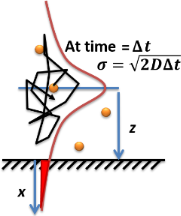
Scheme of molecular diffusion in the solution. Orange dots are solute molecules, solvent molecules are not drawn, black arrow is an example random walk trajectory, and the red curve is the diffusive Gaussian broadening probability function from the Fick's law of diffusion.

The adsorption or absorption rate of a dilute solute to a surface or interface in a (gas or liquid) solution can be calculated using Fick's laws of diffusion. The accumulated number of molecules adsorbed on the surface is expressed by the Langmuir-Schaefer equation at the short-time limit by integrating the diffusion flux equation over time: ^[13]

${\displaystyle \Gamma =2AC{\sqrt {\frac {Dt}{\pi }}}}$

• ${\displaystyle \Gamma }$ is number of molecules in unit # molecules adsorbed during the time ${\displaystyle t}$.
• A is the surface area (m²).
• C is the number concentration of the adsorber molecules in the bulk solution (#/m³).
• D is diffusion coefficient of the adsorber (m²/s).
• t is elapsed time (s).

The equation is named after American chemists Irving Langmuir and Vincent Schaefer.

The Langmuir–Schaefer equation can be extended to the Ward–Tordai Equation to account for the "back-diffusion" of rejected molecules from the surface: ^[14]

${\displaystyle \Gamma =2AC{\sqrt {\frac {Dt}{\pi }}}-A{\sqrt {\frac {D}{\pi }}}\int _{0}^{\sqrt {t}}{\frac {C_{\text{b}}(\tau )}{\sqrt {t-\tau }}}\,d\tau }$

where ${\displaystyle C}$ is the bulk concentration, ${\displaystyle C_{\text{b}}}$ is the sub-surface concentration (which is a function of time depending on the reaction model of the adsorption), and ${\displaystyle \tau }$ is a dummy variable.

Monte Carlo simulations show that these two equations work to predict the adsorption rate of systems that form predictable concentration gradients near the surface but have troubles for systems without or with unpredictable concentration gradients, such as typical biosensing systems or when flow and convection are significant. ^[15]

A brief history of the theories on diffusive adsorption.

A brief history of diffusive adsorption is shown in the right figure. ^[15] A noticeable challenge of understanding the diffusive adsorption at the single-molecule level is the fractal nature of diffusion. Most computer simulations pick a time step for diffusion which ignores the fact that there are self-similar finer diffusion events (fractal) within each step. Simulating the fractal diffusion shows that a factor of two corrections should be introduced for the result of a fixed time-step adsorption simulation, bringing it to be consistent with the above two equations. ^[15]

A more problematic result of the above equations is they predict the lower limit of adsorption under ideal situations but is very difficult to predict the actual adsorption rates. The equations are derived at the long-time-limit condition when a stable concentration gradient has been formed near the surface. But real adsorption is often done much faster than this infinite time limit, i.e., the concentration gradient, decay of concentration at the sub-surface, is only partially formed before the surface has been saturated, thus the adsorption rate measured is almost always faster than the equations have predicted for low or none energy barrier adsorption (unless there is a significant adsorption energy barrier that slows down the absorption significantly), for example, thousands to millions time faster in the self-assembly of monolayers at the water-air or water-substrate interfaces. ^[13] As such, it is necessary to calculate the evolution of the concentration gradient near the surface and find out a proper time to stop the imagined infinite evolution for practical applications. While it is hard to predict when to stop but it is reasonably easy to calculate the shortest time that matters, the critical time when the first nearest neighbor from the substrate surface feels the building-up of the concentration gradient. This yields the upper limit of the adsorption rate under an ideal situation when there are no other factors than diffusion that affect the absorber dynamics: ^[15]

${\displaystyle \langle r\rangle ={\frac {4}{\pi }}Ac_{b}^{4/3}D}$

• ${\displaystyle \langle r\rangle }$ is the adsorption rate assuming under adsorption energy barrier-free situation, in unit #/s.
• ${\displaystyle A}$ is the area of the surface of interest on an "infinite and flat" substrate (m²).
• ${\displaystyle C_{b}}$ is the concentration of the absorber molecule in the bulk solution (#/m³).
• ${\displaystyle D}$ is the diffusion constant of the absorber in the solution (m²/s).
• Dimensional analysis of these units is satisfied.

This equation can be used to predict the initial adsorption rate of any system; It can be used to predict the steady-state adsorption rate of a typical biosensing system when the binding site is just a very small fraction of the substrate surface and a near-surface concentration gradient is never formed; It can also be used to predict the adsorption rate of molecules on the surface when there is a significant flow to push the concentration gradient very shallowly in the sub-surface.

In the ultrashort time limit, in the order of the diffusion time a²/D, where a is the particle radius, the diffusion is described by the Langevin equation. At a longer time, the Langevin equation merges into the Stokes–Einstein equation. The latter is appropriate for the condition of the diluted solution, where long-range diffusion is considered. According to the fluctuation-dissipation theorem based on the Langevin equation in the long-time limit and when the particle is significantly denser than the surrounding fluid, the time-dependent diffusion constant is: ^[16]

${\displaystyle D(t)=\mu \,k_{\rm {B}}T\left(1-e^{-t/(m\mu )}\right)}$

where (all in SI units)

• k_B is the Boltzmann constant
• T is the absolute temperature
• μ is the mobility of the particle in the fluid or gas, which can be calculated using the Einstein relation (kinetic theory)
• m is the mass of the particle
• t is time.

For a single molecule such as organic molecules or biomolecules (e.g. proteins) in water, the exponential term is negligible due to the small product of mμ in the picosecond region.

When the area of interest is the size of a molecule (specifically, a long cylindrical molecule such as DNA), the adsorption rate equation represents the collision frequency of two molecules in a diluted solution, with one molecule a specific side and the other no steric dependence, i.e., a molecule (random orientation) hit one side of the other. The diffusion constant need to be updated to the relative diffusion constant between two diffusing molecules. This estimation is especially useful in studying the interaction between a small molecule and a larger molecule such as a protein. The effective diffusion constant is dominated by the smaller one whose diffusion constant can be used instead.

The above hitting rate equation is also useful to predict the kinetics of molecular self-assembly on a surface. Molecules are randomly oriented in the bulk solution. Assuming 1/6 of the molecules has the right orientation to the surface binding sites, i.e. 1/2 of the z-direction in x, y, z three dimensions, thus the concentration of interest is just 1/6 of the bulk concentration. Put this value into the equation one should be able to calculate the theoretical adsorption kinetic curve using the Langmuir adsorption model. In a more rigid picture, 1/6 can be replaced by the steric factor of the binding geometry.

Comparing collision theory and diffusive collision theory.

The bimolecular collision frequency related to many reactions including protein coagulation/aggregation is initially described by Smoluchowski coagulation equation proposed by Marian Smoluchowski in a seminal 1916 publication, ^[18] derived from Brownian motion and Fick's laws of diffusion. Under an idealized reaction condition for A + B → product in a diluted solution, Smoluchovski suggested that the molecular flux at the infinite time limit can be calculated from Fick's laws of diffusion yielding a fixed/stable concentration gradient from the target molecule, e.g. B is the target molecule holding fixed relatively, and A is the moving molecule that creates a concentration gradient near the target molecule B due to the coagulation reaction between A and B. Smoluchowski calculated the collision frequency between A and B in the solution with unit #/s/m³:

${\displaystyle Z_{AB}=4{\pi }RD_{r}C_{A}C_{B}}$

where,

• ${\displaystyle R}$ is the radius of the collision
• ${\displaystyle D_{r}=D_{A}+D_{B}}$ is the relative diffusion constant between A and B (m²/s)
• ${\displaystyle C_{A}}$ and ${\displaystyle C_{B}}$ are number concentrations of A and B respectively (#/m³).

The reaction order of this bimolecular reaction is 2 which is the analogy to the result from collision theory by replacing the moving speed of the molecule with diffusive flux. In the collision theory, the traveling time between A and B is proportional to the distance which is a similar relationship for the diffusion case if the flux is fixed.

However, under a practical condition, the concentration gradient near the target molecule is evolving over time with the molecular flux evolving as well, ^[15] and on average the flux is much bigger than the infinite time limit flux Smoluchowski has proposed. Thus, this Smoluchowski frequency represents the lower limit of the real collision frequency.

In 2022, Chen calculates the upper limit of the collision frequency between A and B in a solution assuming the bulk concentration of the moving molecule is fixed after the first nearest neighbor of the target molecule. ^[17] Thus the concentration gradient evolution stops at the first nearest neighbor layer given a stop-time to calculate the actual flux. He named this the critical time and derive the diffusive collision frequency in unit #/s/m³: ^[17]

${\displaystyle Z_{AB}={\frac {8}{\pi }}{\sigma }D_{r}C_{A}C_{B}{\sqrt[{3}]{C_{A}+C_{B}}}}$

where,

• ${\displaystyle {\sigma }}$ is the area of the cross-section of the collision (m²).
• ${\displaystyle D_{r}=D_{A}+D_{B}}$ is the relative diffusion constant between A and B (m²/s).
• ${\displaystyle C_{A}}$ and ${\displaystyle C_{B}}$ are number concentrations of A and B respectively (#/m³).

This equation assumes the upper limit of a diffusive collision frequency between A and B is when the first neighbor layer starts to feel the evolution of the concentration gradient, whose reaction order is 2+1/3 instead of 2. Both the Smoluchowski equation and the JChen equation satisfy dimensional checks with SI units. But the former is dependent on the radius and the latter is on the area of the collision sphere. The actual reaction order for a bimolecular unit reaction could be between 2 and 2+1/3, which makes sense because the diffusive collision time is squarely dependent on the distance between the two molecules.

Biological perspective

The first law gives rise to the following formula: ^[19]

${\displaystyle {\text{flux}}={-P\left(c_{2}-c_{1}\right)}}$

in which

• P is the permeability, an experimentally determined membrane "conductance" for a given gas at a given temperature.
• c₂ − c₁ is the difference in concentration of the gas across the membrane for the direction of flow (from c₁ to c₂).

Fick's first law is also important in radiation transfer equations. However, in this context, it becomes inaccurate when the diffusion constant is low and the radiation becomes limited by the speed of light rather than by the resistance of the material the radiation is flowing through. In this situation, one can use a flux limiter.

The exchange rate of a gas across a fluid membrane can be determined by using this law together with Graham's law.

Under the condition of a diluted solution when diffusion takes control, the membrane permeability mentioned in the above section can be theoretically calculated for the solute using the equation mentioned in the last section (use with particular care because the equation is derived for dense solutes, while biological molecules are not denser than water): ^[12]

${\displaystyle P=2A_{p}\eta _{tm}{\sqrt {D/(\pi t)}}}$

where

• ${\displaystyle A_{P}}$ is the total area of the pores on the membrane (unit m²).
• ${\displaystyle \eta _{tm}}$ transmembrane efficiency (unitless), which can be calculated from the stochastic theory of chromatography.
• D is the diffusion constant of the solute unit m²⋅s⁻¹.
• t is time unit s.
• c₂, c₁ concentration should use unit mol m⁻³, so flux unit becomes mol s⁻¹.

The flux is decay over the square root of time because a concentration gradient builds up near the membrane over time under ideal conditions. When there is flow and convection, the flux can be significantly different than the equation predicts and show an effective time t with a fixed value, ^[15] which makes the flux stable instead of decay over time. A critical time has been estimated under idealized flow conditions when there is no gradient formed. ^{[15] [17]} This strategy is adopted in biology such as blood circulation.

Semiconductor fabrication applications

The semiconductor is a collective term for a series of devices. It mainly includes three categories：two-terminal devices, three-terminal devices, and four-terminal devices. The combination of the semiconductors is called an integrated circuit.

The relationship between Fick's law and semiconductors: the principle of the semiconductor is transferring chemicals or dopants from a layer to a layer. Fick's law can be used to control and predict the diffusion by knowing how much the concentration of the dopants or chemicals move per meter and second through mathematics.

Therefore, different types and levels of semiconductors can be fabricated.

Integrated circuit fabrication technologies, model processes like CVD, thermal oxidation, wet oxidation, doping, etc. use diffusion equations obtained from Fick's law.

CVD method of fabricate semiconductor

The wafer is a kind of semiconductor whose silicon substrate is coated with a layer of CVD-created polymer chain and films. This film contains n-type and p-type dopants and takes responsibility for dopant conductions. The principle of CVD relies on the gas phase and gas-solid chemical reaction to create thin films.

The viscous flow regime of CVD is driven by a pressure gradient. CVD also includes a diffusion component distinct from the surface diffusion of adatoms. In CVD, reactants and products must also diffuse through a boundary layer of stagnant gas that exists next to the substrate. The total number of steps required for CVD film growth are gas phase diffusion of reactants through the boundary layer, adsorption and surface diffusion of adatoms, reactions on the substrate, and gas phase diffusion of products away through the boundary layer.

The velocity profile for gas flow is:

$${\displaystyle \delta (x)=\left({\frac {5x}{\mathrm {Re} ^{1/2}}}\right)\mathrm {Re} ={\frac {v\rho L}{\eta }}}$$

where

• ${\displaystyle \delta }$ is the thickness
• ${\displaystyle \mathrm {Re} }$ is the Reynolds number
• x is the length of the subtrate
• v = 0 at any surface
• ${\displaystyle \eta }$ is viscosity
• ${\displaystyle \rho }$ is density.

Integrated the x from 0 to L, it gives the average thickness:

$${\displaystyle \delta ={\frac {10L}{3\mathrm {Re} ^{1/2}}}}$$

To keep the reaction balanced, reactants must diffuse through the stagnant boundary layer to reach the substrate. So a thin boundary layer is desirable. According to the equations, increasing vo would result in more wasted reactants. The reactants will not reach the substrate uniformly if the flow becomes turbulent. Another option is to switch to a new carrier gas with lower viscosity or density.

The Fick's first law describes diffusion through the boundary layer. As a function of pressure (P) and temperature (T) in a gas, diffusion is determined.

$${\displaystyle D=D_{0}\left({\frac {P_{0}}{P}}\right)\left({\frac {T}{T_{0}}}\right)^{3/2}}$$

where

• ${\displaystyle P_{0}}$ is the standard pressure
• ${\displaystyle T_{0}}$ is the standard temperature
• ${\displaystyle D_{0}}$ is the standard diffusitivity.

The equation tells that increasing the temperature or decreasing the pressure can increase the diffusivity.

Fick's first law predicts the flux of the reactants to the substrate and product away from the substrate:

$${\displaystyle J=-D_{i}\left({\frac {dc_{i}}{dx}}\right)}$$

where

• ${\displaystyle x}$ is the thickness ${\displaystyle \delta }$
• ${\displaystyle dc_{i}}$ is the first reactant's concentration.

In ideal gas law ${\displaystyle PV=nRT}$, the concentration of the gas is expressed by partial pressure.

$${\displaystyle J=-D_{i}\left({\frac {P_{i}-P_{0}}{\delta RT}}\right)}$$

where

• ${\displaystyle R}$ is the gas constant
• ${\displaystyle {\frac {P_{i}-P_{0}}{\delta }}}$ is the partial pressure gradient.

As a result, Fick's first law tells us we can use a partial pressure gradient to control the diffusivity and control the growth of thin films of semiconductors.

In many realistic situations, the simple Fick's law is not an adequate formulation for the semiconductor problem. It only applies to certain conditions, for example, given the semiconductor boundary conditions: constant source concentration diffusion, limited source concentration, or moving boundary diffusion (where junction depth keeps moving into the substrate).

Invalidity of Fickian diffusion

It is important to note that, even though Fickian diffusion has been used to model diffusion processes in semiconductor manufacturing (including CVD reactors) in early days, it often fails to validate the diffusion in advanced semiconductor nodes (< 90 nm). This mostly stems from the inability of Fickian diffusion to model diffusion processes accurately at molecular level and smaller. In advanced semiconductor manufacturing, it is important to understand the movement at atomic scales, which is failed by continuum diffusion. Today, most semiconductor manufacturers use random walk to study and model diffusion processes. This allows us to study the effects of diffusion in a discrete manner to understand the movement of individual atoms, molecules, plasma etc.

In such a process, the movements of diffusing species (atoms, molecules, plasma etc.) are treated as a discrete entity, following a random walk through the CVD reactor, boundary layer, material structures etc. Sometimes, the movements might follow a biased-random walk depending on the processing conditions. Statistical analysis is done to understand variation/stochasticity arising from the random walk of the species, which in-turn affects the overall process and electrical variations.

Food production and cooking

The formulation of Fick's first law can explain a variety of complex phenomena in the context of food and cooking: Diffusion of molecules such as ethylene promotes plant growth and ripening, salt and sugar molecules promotes meat brining and marinating, and water molecules promote dehydration. Fick's first law can also be used to predict the changing moisture profiles across a spaghetti noodle as it hydrates during cooking. These phenomena are all about the spontaneous movement of particles of solutes driven by the concentration gradient. In different situations, there is different diffusivity which is a constant. ^[20]

By controlling the concentration gradient, the cooking time, shape of the food, and salting can be controlled.

See also

• Advection
• Churchill–Bernstein equation
• Diffusion
• False diffusion
• Gas exchange
• Mass flux
• Maxwell–Stefan diffusion
• Nernst–Planck equation
• Osmosis

Citations

1. "Molecular Diffusion - an overview | ScienceDirect Topics". www.sciencedirect.com. Retrieved 26 February 2024.
2. • Fick A (1855). "Ueber Diffusion". Annalen der Physik (in German). 94 (1): 59–86. Bibcode:1855AnP...170...59F. doi: 10.1002/andp.18551700105 .
   • Fick A (1855). "On liquid diffusion". The London, Edinburgh, and Dublin Philosophical Magazine and Journal of Science. 10 (63): 30–39. doi:10.1080/14786445508641925.
3. Philibert J (2005). "One and a Half Centuries of Diffusion: Fick, Einstein, before and beyond" (PDF). Diffusion Fundamentals. 2: 1.1–1.10. Archived from the original (PDF) on 5 February 2009.
4. Vázquez JL (2006). "The Porous Medium Equation". Mathematical Theory. Oxford Univ. Press.
5. Gorban AN, Sargsyan HP, Wahab HA (2011). "Quasichemical Models of Multicomponent Nonlinear Diffusion". Mathematical Modelling of Natural Phenomena. 6 (5): 184–262. arXiv: 1012.2908 . doi:10.1051/mmnp/20116509. S2CID   18961678.
6. Atkins P, de Paula J (2006). Physical Chemistry for the Life Science.
7. Conlisk AT (2013). Essentials of Micro- and Nanofluidics: With Applications to the Biological and Chemical Sciences. Cambridge University Press. p. 43. ISBN   9780521881685.
8. Williams FA (1985). "Appendix E". Combustion Theory. Benjamin/Cummings.
9. "Fickian Diffusion - an overview | ScienceDirect Topics". www.sciencedirect.com. Retrieved 11 May 2022.
10. Taylor R, Krishna R (1993). Multicomponent mass transfer. Wiley Series in Chemical Engineering. Vol. 2. John Wiley & Sons. ISBN   978-0-471-57417-0.
11. Brogioli D, Vailati A (January 2001). "Diffusive mass transfer by nonequilibrium fluctuations: Fick's law revisited". Physical Review E. 63 (1 Pt 1): 012105. arXiv: cond-mat/0006163 . Bibcode:2000PhRvE..63a2105B. doi:10.1103/PhysRevE.63.012105. PMID   11304296. S2CID   1302913.
12. Pyle JR, Chen J (2 November 2017). "Photobleaching of YOYO-1 in super-resolution single DNA fluorescence imaging". Beilstein Journal of Nanotechnology. 8: 2296–2306. doi:10.3762/bjnano.8.229. PMC   5687005 . PMID   29181286.
13. Langmuir I, Schaefer VJ (1937). "The Effect of Dissolved Salts on Insoluble Monolayers". Journal of the American Chemical Society. 29 (11): 2400–2414. doi:10.1021/ja01290a091.
14. Ward AF, Tordai L (1946). "Time-dependence of Boundary Tensions of Solutions I. The Role of Diffusion in Time-effects". Journal of Chemical Physics. 14 (7): 453–461. Bibcode:1946JChPh..14..453W. doi:10.1063/1.1724167.
15. Chen J (January 2022). "Simulating stochastic adsorption of diluted solute molecules at interfaces". AIP Advances. 12 (1): 015318. Bibcode:2022AIPA...12a5318C. doi:10.1063/5.0064140. PMC   8758205 . PMID   35070490.
16. Bian X, Kim C, Karniadakis GE (August 2016). "111 years of Brownian motion". Soft Matter. 12 (30): 6331–6346. Bibcode:2016SMat...12.6331B. doi:10.1039/c6sm01153e. PMC   5476231 . PMID   27396746.
17. Chen J (December 2022). "Why Should the Reaction Order of a Bimolecular Reaction be 2.33 Instead of 2?". The Journal of Physical Chemistry A. 126 (51): 9719–9725. Bibcode:2022JPCA..126.9719C. doi:10.1021/acs.jpca.2c07500. PMC   9805503 . PMID   36520427.
18. Smoluchowski M (1916). "Drei Vorträge über Diffusion, Brownsche Molekularbewegung und Koagulation von Kolloidteilchen". Zeitschrift für Physik (in German). 17: 557–571, 585–599. Bibcode:1916ZPhy...17..557S.
19. Nosek TM. "Section 3/3ch9/s3ch9_2". Essentials of Human Physiology. Archived from the original on 24 March 2016.
20. Zhou L, Nyberg K, Rowat AC (September 2015). "Understanding diffusion theory and Fick's law through food and cooking". Advances in Physiology Education. 39 (3): 192–197. doi:10.1152/advan.00133.2014. PMID   26330037. S2CID   3921833.

Further reading

• Berg HC (1977). Random Walks in Biology. Princeton.
• Bird RB, Stewart WE, Lightfoot EN (1976). Transport Phenomena. John Wiley & Sons.
• Bokshtein BS, Mendelev MI, Srolovitz DJ, eds. (2005). Thermodynamics and Kinetics in Materials Science: A Short Course . Oxford: Oxford University Press. pp.  167–171.
• Crank J (1980). The Mathematics of Diffusion. Oxford University Press.
• Fick A (1855). "On liquid diffusion". Annalen der Physik und Chemie. 94: 59. – reprinted in Fick, Adolph (1995). "On liquid diffusion". Journal of Membrane Science. 100: 33–38. doi:10.1016/0376-7388(94)00230-v.
• Smith WF (2004). Foundations of Materials Science and Engineering (3rd ed.). McGraw-Hill.

External links

• Fick's equations, Boltzmann's transformation, etc. (with figures and animations)
• Fick's Second Law on OpenStax