Gravitational lensing formalism

For broader coverage of this topic, see Gravitational lens.

In general relativity, a point mass deflects a light ray with impact parameter ${\displaystyle b~}$ by an angle approximately equal to

${\displaystyle {\hat {\alpha }}={\frac {4GM}{c^{2}b}}}$

where G is the gravitational constant, M the mass of the deflecting object and c the speed of light. A naive application of Newtonian gravity can yield exactly half this value, where the light ray is assumed as a massed particle and scattered by the gravitational potential well. This approximation is good when ${\displaystyle 4GM/c^{2}b}$ is small.

In situations where general relativity can be approximated by linearized gravity, the deflection due to a spatially extended mass can be written simply as a vector sum over point masses. In the continuum limit, this becomes an integral over the density ${\displaystyle \rho ~}$, and if the deflection is small we can approximate the gravitational potential along the deflected trajectory by the potential along the undeflected trajectory, as in the Born approximation in quantum mechanics. The deflection is then

${\displaystyle {\vec {\hat {\alpha }}}({\vec {\xi }})={\frac {4G}{c^{2}}}\int d^{2}\xi ^{\prime }\int dz\rho ({\vec {\xi }}^{\prime },z){\frac {\vec {b}}{|{\vec {b}}|^{2}}},~{\vec {b}}\equiv {\vec {\xi }}-{\vec {\xi ^{\prime }}}}$

where ${\displaystyle z}$ is the line-of-sight coordinate, and ${\displaystyle {\vec {b}}}$ is the vector impact parameter of the actual ray path from the infinitesimal mass ${\displaystyle d^{2}\xi ^{\prime }dz\rho ({\vec {\xi }}^{\prime },z)}$ located at the coordinates ${\displaystyle ({\vec {\xi }}^{\prime },z)}$. ^[1]

Thin lens approximation

In the limit of a "thin lens", where the distances between the source, lens, and observer are much larger than the size of the lens (this is almost always true for astronomical objects), we can define the projected mass density

${\displaystyle \Sigma ({\vec {\xi }}^{\prime })=\int \rho ({\vec {\xi }}^{\prime },z)dz}$

where ${\displaystyle {\vec {\xi }}^{\prime }}$ is a vector in the plane of the sky. The deflection angle is then

${\displaystyle {\vec {\hat {\alpha }}}({\vec {\xi }})={\frac {4G}{c^{2}}}\int {\frac {({\vec {\xi }}-{\vec {\xi }}^{\prime })\Sigma ({\vec {\xi }}^{\prime })}{|{\vec {\xi }}-{\vec {\xi }}^{\prime }|^{2}}}d^{2}\xi ^{\prime }}$

Angles involved in a thin gravitational lens system.

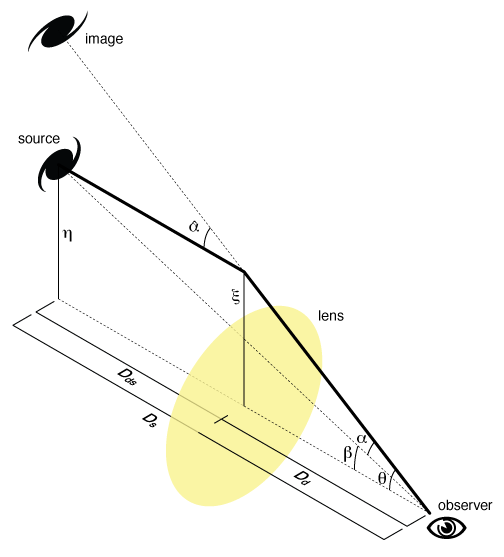
As shown in the diagram on the right, the difference between the unlensed angular position ${\displaystyle {\vec {\beta }}}$ and the observed position ${\displaystyle {\vec {\theta }}}$ is this deflection angle, reduced by a ratio of distances, described as the lens equation

${\displaystyle {\vec {\beta }}={\vec {\theta }}-{\vec {\alpha }}({\vec {\theta }})={\vec {\theta }}-{\frac {D_{ds}}{D_{s}}}{\vec {\hat {\alpha }}}(D_{d}{\vec {\theta }})}$

where ${\displaystyle D_{ds}~}$ is the distance from the lens to the source, ${\displaystyle D_{s}~}$ is the distance from the observer to the source, and ${\displaystyle D_{d}~}$ is the distance from the observer to the lens. For extragalactic lenses, these must be angular diameter distances.

In strong gravitational lensing, this equation can have multiple solutions, because a single source at ${\displaystyle {\vec {\beta }}}$ can be lensed into multiple images.

Convergence and deflection potential

The reduced deflection angle ${\displaystyle {\vec {\alpha }}({\vec {\theta }})}$ can be written as

${\displaystyle {\vec {\alpha }}({\vec {\theta }})={\frac {1}{\pi }}\int d^{2}\theta ^{\prime }{\frac {({\vec {\theta }}-{\vec {\theta }}^{\prime })\kappa ({\vec {\theta }}^{\prime })}{|{\vec {\theta }}-{\vec {\theta }}^{\prime }|^{2}}}}$

where we define the convergence

${\displaystyle \kappa ({\vec {\theta }})={\frac {\Sigma ({\vec {\theta }})}{\Sigma _{cr}}}}$

and the critical surface density (not to be confused with the critical density of the universe)

${\displaystyle \Sigma _{cr}={\frac {c^{2}D_{s}}{4\pi GD_{ds}D_{d}}}}$

We can also define the deflection potential

${\displaystyle \psi ({\vec {\theta }})={\frac {1}{\pi }}\int d^{2}\theta ^{\prime }\kappa ({\vec {\theta }}^{\prime })\ln |{\vec {\theta }}-{\vec {\theta }}^{\prime }|}$

such that the scaled deflection angle is just the gradient of the potential and the convergence is half the Laplacian of the potential:

${\displaystyle {\vec {\theta }}-{\vec {\beta }}={\vec {\alpha }}({\vec {\theta }})={\vec {\nabla }}\psi ({\vec {\theta }})}$

${\displaystyle \kappa ({\vec {\theta }})={\frac {1}{2}}\nabla ^{2}\psi ({\vec {\theta }})}$

The deflection potential can also be written as a scaled projection of the Newtonian gravitational potential ${\displaystyle \Phi ~}$ of the lens ^[2]

${\displaystyle \psi ({\vec {\theta }})={\frac {2D_{ds}}{D_{d}D_{s}c^{2}}}\int \Phi (D_{d}{\vec {\theta }},z)dz}$

Lensing Jacobian

The Jacobian between the unlensed and lensed coordinate systems is

${\displaystyle A_{ij}={\frac {\partial \beta _{i}}{\partial \theta _{j}}}=\delta _{ij}-{\frac {\partial \alpha _{i}}{\partial \theta _{j}}}=\delta _{ij}-{\frac {\partial ^{2}\psi }{\partial \theta _{i}\partial \theta _{j}}}}$

where ${\displaystyle \delta _{ij}~}$ is the Kronecker delta. Because the matrix of second derivatives must be symmetric, the Jacobian can be decomposed into a diagonal term involving the convergence and a trace-free term involving the shear${\displaystyle \gamma ~}$

${\displaystyle A=(1-\kappa )\left[{\begin{array}{c c }1&0\\0&1\end{array}}\right]-\gamma \left[{\begin{array}{c c }\cos 2\phi &\sin 2\phi \\\sin 2\phi &-\cos 2\phi \end{array}}\right]}$

where ${\displaystyle \phi ~}$ is the angle between ${\displaystyle {\vec {\alpha }}}$ and the x-axis. The term involving the convergence magnifies the image by increasing its size while conserving surface brightness. The term involving the shear stretches the image tangentially around the lens, as discussed in weak lensing observables.

The shear defined here is not equivalent to the shear traditionally defined in mathematics, though both stretch an image non-uniformly.

Effect of the components of convergence and shear on a circular source represented by the solid green circle. The complex shear notation is defined below.

Fermat surface

There is an alternative way of deriving the lens equation, starting from the photon arrival time (Fermat surface)

${\displaystyle t=\int _{0}^{z_{s}}{ndz \over c\cos \alpha (z)}}$

where ${\displaystyle dz/c}$ is the time to travel an infinitesimal line element along the source-observer straight line in vacuum, which is then corrected by the factor

${\displaystyle 1/\cos(\alpha (z))\approx 1+{\alpha (z)^{2} \over 2}}$

to get the line element along the bended path ${\displaystyle dl={dz \over c\cos \alpha (z)}}$ with a varying small pitch angle ${\displaystyle \alpha (z),}$ and the refraction index n for the "aether", i.e., the gravitational field. The last can be obtained from the fact that a photon travels on a null geodesic of a weakly perturbed static Minkowski universe

${\displaystyle ds^{2}=0=c^{2}dt^{2}\left(1+{2\Phi \over c^{2}}\right)-\left(1+{2\Phi \over c^{2}}\right)^{-1}dl^{2}}$

where the uneven gravitational potential ${\displaystyle \Phi \ll c^{2}}$ drives a changing the speed of light

${\displaystyle c'={dl/dt}=\left(1+{2\Phi \over c^{2}}\right)c.}$

So the refraction index

${\displaystyle n\equiv {c \over c'}\approx \left(1-{2\Phi \over c^{2}}\right).}$

The refraction index greater than unity because of the negative gravitational potential ${\displaystyle \Phi }$.

Put these together and keep the leading terms we have the time arrival surface

${\displaystyle t\approx \int _{0}^{z_{s}}{dz \over c}+\int _{0}^{z_{s}}{dz \over c}{\alpha (z)^{2} \over 2}-\int _{0}^{z_{s}}{dz \over c}{2\Phi \over c^{2}}.}$

The first term is the straight path travel time, the second term is the extra geometric path, and the third is the gravitational delay. Make the triangle approximation that ${\displaystyle \alpha (z)=\theta -\beta }$ for the path between the observer and the lens, and ${\displaystyle \alpha (z)\approx (\theta -\beta ){D_{d} \over D_{ds}}}$ for the path between the lens and the source. The geometric delay term becomes

${\displaystyle {D_{d} \over c}{({\vec {\theta }}-{\vec {\beta }})^{2} \over 2}+{D_{ds} \over c}{\left[({\vec {\theta }}-{\vec {\beta }}){D_{d} \over D_{ds}}\right]^{2} \over 2}={D_{d}D_{s} \over D_{ds}c}{({\vec {\theta }}-{\vec {\beta }})^{2} \over 2}.}$

(How? There is no ${\displaystyle D_{s}}$ on the left. Angular diameter distances don't add in a simple way, in general.) So the Fermat surface becomes

${\displaystyle t=constant+{D_{d}D_{s} \over D_{ds}c}\tau ,~\tau \equiv \left[{({\vec {\theta }}-{\vec {\beta }})^{2} \over 2}-\psi \right]}$

where ${\displaystyle \tau }$ is so-called dimensionless time delay, and the 2D lensing potential

${\displaystyle \psi ({\vec {\theta }})={\frac {2D_{ds}}{D_{d}D_{s}c^{2}}}\int \Phi (D_{d}{\vec {\theta }},z)dz.}$

The images lie at the extrema of this surface, so the variation of ${\displaystyle \tau }$ with ${\displaystyle {\vec {\theta }}}$ is zero,

${\displaystyle 0=\nabla _{\vec {\theta }}\tau ={\vec {\theta }}-{\vec {\beta }}-\nabla _{\vec {\theta }}\psi ({\vec {\theta }})}$

which is the lens equation. Take the Poisson's equation for 3D potential

${\displaystyle \Phi ({\vec {\xi }})=-\int {\frac {d^{3}\xi ^{\prime }\rho ({\vec {\xi }}^{\prime })}{|{\vec {\xi }}-{\vec {\xi }}^{\prime }|}}}$

and we find the 2D lensing potential

${\displaystyle \psi ({\vec {\theta }})=-{\frac {2GD_{ds}}{D_{d}D_{s}c^{2}}}\int dz\int {\frac {d^{3}\xi ^{\prime }\rho ({\vec {\xi }}^{\prime })}{|{\vec {\xi }}-{\vec {\xi }}^{\prime }|}}=-\sum _{i}{\frac {2GM_{i}D_{is}}{D_{s}D_{i}c^{2}}}\left[\sinh ^{-1}{|z-D_{i}| \over D_{i}|{\vec {\theta }}-{\vec {\theta }}_{i}|}\right]|_{D_{i}}^{D_{s}}+|_{D_{i}}^{0}.}$

Here we assumed the lens is a collection of point masses ${\displaystyle M_{i}}$ at angular coordinates ${\displaystyle {\vec {\theta }}_{i}}$ and distances ${\displaystyle z=D_{i}.}$ Use ${\displaystyle \sinh ^{-1}1/x=\ln(1/x+{\sqrt {1/x^{2}+1}})\approx -\ln(x/2)}$ for very small x we find

${\displaystyle \psi ({\vec {\theta }})\approx \sum _{i}{\frac {4GM_{i}D_{is}}{D_{s}D_{i}c^{2}}}\left[\ln \left({|{\vec {\theta }}-{\vec {\theta }}_{i}| \over 2}{D_{i} \over D_{is}}\right)\right].}$

One can compute the convergence by applying the 2D Laplacian of the 2D lensing potential

${\displaystyle \kappa ({\vec {\theta }})={\frac {1}{2}}\nabla _{\vec {\theta }}^{2}\psi ({\vec {\theta }})={\frac {4\pi GD_{ds}D_{d}}{c^{2}D_{s}}}\int dz\rho (D_{d}{\vec {\theta }},z)={\Sigma \over \Sigma _{cr}}=\sum _{i}{4\pi GM_{i}D_{is} \over c^{2}D_{i}D_{s}}\delta ({\vec {\theta }}-{\vec {\theta }}_{i})}$

in agreement with earlier definition ${\displaystyle \kappa ({\vec {\theta }})={\Sigma \over \Sigma _{cr}}}$ as the ratio of projected density with the critical density. Here we used ${\displaystyle \nabla ^{2}1/r=-4\pi \delta (r)}$ and ${\displaystyle \nabla _{\vec {\theta }}=D_{d}\nabla .}$

We can also confirm the previously defined reduced deflection angle

${\displaystyle {\vec {\theta }}-{\vec {\beta }}=\nabla _{\vec {\theta }}\psi ({\vec {\theta }})=\sum _{i}{\theta _{Ei}^{2} \over |{\vec {\theta }}-{\vec {\theta }}_{i}|},~\pi \theta _{Ei}^{2}\equiv {4\pi GM_{i}D_{is} \over c^{2}D_{s}D_{i}}}$

where ${\displaystyle \theta _{Ei}}$ is the so-called Einstein angular radius of a point lens ${\displaystyle M_{i}}$. For a single point lens at the origin we recover the standard result that there will be two images at the two solutions of the essentially quadratic equation

${\displaystyle {\vec {\theta }}-{\vec {\beta }}={\theta _{E}^{2} \over |{\vec {\theta }}|}.}$

The amplification matrix can be obtained by double derivatives of the dimensionless time delay

${\displaystyle A_{ij}={\partial \beta _{j} \over \partial \theta _{i}}={\partial \tau \over \partial \theta _{i}\partial \theta _{j}}=\delta _{ij}-{\partial \psi \over \partial \theta _{i}\partial \theta _{j}}=\left[{\begin{array}{c c }1-\kappa -\gamma _{1}&\gamma _{2}\\\gamma _{2}&1-\kappa +\gamma _{1}\end{array}}\right]}$

where we have define the derivatives

${\displaystyle \kappa ={\partial \psi \over 2\partial \theta _{1}\partial \theta _{1}}+{\partial \psi \over 2\partial \theta _{2}\partial \theta _{2}},~\gamma _{1}\equiv {\partial \psi \over 2\partial \theta _{1}\partial \theta _{1}}-{\partial \psi \over 2\partial \theta _{2}\partial \theta _{2}},~\gamma _{2}\equiv {\partial \psi \over \partial \theta _{1}\partial \theta _{2}}}$

which takes the meaning of convergence and shear. The amplification is the inverse of the Jacobian

${\displaystyle A=1/det(A_{ij})={1 \over (1-\kappa )^{2}-\gamma _{1}^{2}-\gamma _{2}^{2}}}$

where a positive ${\displaystyle A}$ means either a maxima or a minima, and a negative ${\displaystyle A}$ means a saddle point in the arrival surface.

For a single point lens, one can show (albeit a lengthy calculation) that

${\displaystyle \kappa =0,~\gamma ={\sqrt {\gamma _{1}^{2}+\gamma _{2}^{2}}}={\theta _{E}^{2} \over |\theta |^{2}},~\theta _{E}^{2}={4GMD_{ds} \over c^{2}D_{d}D_{s}}.}$

So the amplification of a point lens is given by

${\displaystyle A=\left(1-{\theta _{E}^{4} \over \theta ^{4}}\right)^{-1}.}$

Note A diverges for images at the Einstein radius ${\displaystyle \theta _{E}.}$

In cases there are multiple point lenses plus a smooth background of (dark) particles of surface density ${\displaystyle \Sigma _{\rm {cr}}\kappa _{\rm {smooth}},}$ the time arrival surface is

${\displaystyle \psi ({\vec {\theta }})\approx {1 \over 2}\kappa _{\rm {smooth}}|\theta |^{2}+\sum _{i}\theta _{E}^{2}\left[\ln \left({|{\vec {\theta }}-{\vec {\theta }}_{i}|^{2} \over 4}{D_{d} \over D_{ds}}\right)\right].}$

To compute the amplification, e.g., at the origin (0,0), due to identical point masses distributed at ${\displaystyle (\theta _{xi},\theta _{yi})}$ we have to add up the total shear, and include a convergence of the smooth background,

${\displaystyle A=\left[(1-\kappa _{\rm {smooth}})^{2}-\left(\sum _{i}{(\theta _{xi}^{2}-\theta _{yi}^{2})\theta _{E}^{2} \over (\theta _{xi}^{2}+\theta _{yi}^{2})^{2}}\right)^{2}-\left(\sum _{i}{(2\theta _{xi}\theta _{yi})\theta _{E}^{2} \over (\theta _{xi}^{2}+\theta _{yi}^{2})^{2}}\right)^{2}\right]^{-1}}$

This generally creates a network of critical curves, lines connecting image points of infinite amplification.

General weak lensing

In weak lensing by large-scale structure, the thin-lens approximation may break down, and low-density extended structures may not be well approximated by multiple thin-lens planes. In this case, the deflection can be derived by instead assuming that the gravitational potential is slowly varying everywhere (for this reason, this approximation is not valid for strong lensing). This approach assumes the universe is well described by a Newtonian-perturbed FRW metric, but it makes no other assumptions about the distribution of the lensing mass.

As in the thin-lens case, the effect can be written as a mapping from the unlensed angular position ${\displaystyle {\vec {\beta }}}$ to the lensed position ${\displaystyle {\vec {\theta }}}$. The Jacobian of the transform can be written as an integral over the gravitational potential ${\displaystyle \Phi ~}$ along the line of sight ^[3]

${\displaystyle {\frac {\partial \beta _{i}}{\partial \theta _{j}}}=\delta _{ij}+\int _{0}^{r_{\infty }}drg(r){\frac {\partial ^{2}\Phi ({\vec {x}}(r))}{\partial x^{i}\partial x^{j}}}}$

where ${\displaystyle r~}$ is the comoving distance, ${\displaystyle x^{i}~}$ are the transverse distances, and

${\displaystyle g(r)=2r\int _{r}^{r_{\infty }}dr'\left(1-{\frac {r^{\prime }}{r}}\right)W(r^{\prime })}$

is the lensing kernel, which defines the efficiency of lensing for a distribution of sources ${\displaystyle W(r)~}$.

The Jacobian ${\displaystyle A_{ij}~}$ can be decomposed into convergence and shear terms just as with the thin-lens case, and in the limit of a lens that is both thin and weak, their physical interpretations are the same.

Weak lensing observables

In weak gravitational lensing, the Jacobian is mapped out by observing the effect of the shear on the ellipticities of background galaxies. This effect is purely statistical; the shape of any galaxy will be dominated by its random, unlensed shape, but lensing will produce a spatially coherent distortion of these shapes.

Measures of ellipticity

In most fields of astronomy, the ellipticity is defined as ${\displaystyle 1-q~}$, where ${\displaystyle q={\frac {b}{a}}}$ is the axis ratio of the ellipse. In weak gravitational lensing, two different definitions are commonly used, and both are complex quantities which specify both the axis ratio and the position angle ${\displaystyle \phi ~}$:

${\displaystyle \chi ={\frac {1-q^{2}}{1+q^{2}}}e^{2i\phi }={\frac {a^{2}-b^{2}}{a^{2}+b^{2}}}e^{2i\phi }}$

${\displaystyle \epsilon ={\frac {1-q}{1+q}}e^{2i\phi }={\frac {a-b}{a+b}}e^{2i\phi }}$

Like the traditional ellipticity, the magnitudes of both of these quantities range from 0 (circular) to 1 (a line segment). The position angle is encoded in the complex phase, but because of the factor of 2 in the trigonometric arguments, ellipticity is invariant under a rotation of 180 degrees. This is to be expected; an ellipse is unchanged by a 180° rotation. Taken as imaginary and real parts, the real part of the complex ellipticity describes the elongation along the coordinate axes, while the imaginary part describes the elongation at 45° from the axes.

The ellipticity is often written as a two-component vector instead of a complex number, though it is not a true vector with regard to transforms:

${\displaystyle \chi =\{\left|\chi \right|\cos 2\phi ,\left|\chi \right|\sin 2\phi \}}$

${\displaystyle \epsilon =\{\left|\epsilon \right|\cos 2\phi ,\left|\epsilon \right|\sin 2\phi \}}$

Real astronomical background sources are not perfect ellipses. Their ellipticities can be measured by finding a best-fit elliptical model to the data, or by measuring the second moments of the image about some centroid ${\displaystyle ({\bar {x}},{\bar {y}})}$

${\displaystyle q_{xx}={\frac {\sum (x-{\bar {x}})^{2}I(x,y)}{\sum I(x,y)}}}$

${\displaystyle q_{yy}={\frac {\sum (y-{\bar {y}})^{2}I(x,y)}{\sum I(x,y)}}}$

${\displaystyle q_{xy}={\frac {\sum (x-{\bar {x}})(y-{\bar {y}})I(x,y)}{\sum I(x,y)}}}$

The complex ellipticities are then

${\displaystyle \chi ={\frac {q_{xx}-q_{yy}+2iq_{xy}}{q_{xx}+q_{yy}}}}$

${\displaystyle \epsilon ={\frac {q_{xx}-q_{yy}+2iq_{xy}}{q_{xx}+q_{yy}+2{\sqrt {q_{xx}q_{yy}-q_{xy}^{2}}}}}}$

This can be used to relate the second moments to traditional ellipse parameters:

${\displaystyle q_{xx}=a^{2}\cos ^{2}\theta +b^{2}\sin ^{2}\theta \,}$

${\displaystyle q_{yy}=a^{2}\sin ^{2}\theta +b^{2}\cos ^{2}\theta \,}$

${\displaystyle q_{xy}=(a^{2}-b^{2})\sin \theta \cos \theta \,}$

and in reverse:

${\displaystyle a^{2}={\frac {q_{xx}+q_{yy}+{\sqrt {(q_{xx}-q_{yy})^{2}+4q_{xy}^{2}}}}{2}}}$

${\displaystyle b^{2}={\frac {q_{xx}+q_{yy}-{\sqrt {(q_{xx}-q_{yy})^{2}+4q_{xy}^{2}}}}{2}}}$

${\displaystyle \tan 2\theta ={\frac {2q_{xy}}{q_{xx}-q_{yy}}}}$

The unweighted second moments above are problematic in the presence of noise, neighboring objects, or extended galaxy profiles, so it is typical to use apodized moments instead:

${\displaystyle q_{xx}={\frac {\sum (x-{\bar {x}})^{2}w(x-{\bar {x}},y-{\bar {y}})I(x,y)}{\sum w(x-{\bar {x}},y-{\bar {y}})I(x,y)}}}$

${\displaystyle q_{yy}={\frac {\sum (y-{\bar {y}})^{2}w(x-{\bar {x}},y-{\bar {y}})I(x,y)}{\sum w(x-{\bar {x}},y-{\bar {y}})I(x,y)}}}$

${\displaystyle q_{xy}={\frac {\sum (x-{\bar {x}})(y-{\bar {y}})w(x-{\bar {x}},y-{\bar {y}})I(x,y)}{\sum w(x-{\bar {x}},y-{\bar {y}})I(x,y)}}}$

Here ${\displaystyle w(x,y)~}$ is a weight function that typically goes to zero or quickly approaches zero at some finite radius.

Image moments cannot generally be used to measure the ellipticity of galaxies without correcting for observational effects, particularly the point spread function. ^[4]

Shear and reduced shear

Recall that the lensing Jacobian can be decomposed into shear ${\displaystyle \gamma ~}$ and convergence ${\displaystyle \kappa ~}$. Acting on a circular background source with radius ${\displaystyle R~}$, lensing generates an ellipse with major and minor axes

${\displaystyle a={\frac {R}{1-\kappa -\gamma }}}$

${\displaystyle b={\frac {R}{1-\kappa +\gamma }}}$

as long as the shear and convergence do not change appreciably over the size of the source (in that case, the lensed image is not an ellipse). Galaxies are not intrinsically circular, however, so it is necessary to quantify the effect of lensing on a non-zero ellipticity.

We can define the complex shear in analogy to the complex ellipticities defined above

${\displaystyle \gamma =\left|\gamma \right|e^{2i\phi }}$

as well as the reduced shear

${\displaystyle g\equiv {\frac {\gamma }{1-\kappa }}}$

The lensing Jacobian can now be written as

${\displaystyle A=\left[{\begin{array}{c c }1-\kappa -\mathrm {Re} [\gamma ]&-\mathrm {Im} [\gamma ]\\-\mathrm {Im} [\gamma ]&1-\kappa +\mathrm {Re} [\gamma ]\end{array}}\right]=(1-\kappa )\left[{\begin{array}{c c }1-\mathrm {Re} [g]&-\mathrm {Im} [g]\\-\mathrm {Im} [g]&1+\mathrm {Re} [g]\end{array}}\right]}$

For a reduced shear ${\displaystyle g~}$ and unlensed complex ellipticities ${\displaystyle \chi _{s}~}$ and ${\displaystyle \epsilon _{s}~}$, the lensed ellipticities are

${\displaystyle \chi ={\frac {\chi _{s}+2g+g^{2}\chi _{s}^{*}}{1+|g|^{2}+2\mathrm {Re} (g\chi _{s}^{*})}}}$

${\displaystyle \epsilon ={\frac {\epsilon _{s}+g}{1+g^{*}\epsilon _{s}}}}$

In the weak lensing limit, ${\displaystyle \gamma \ll 1}$ and ${\displaystyle \kappa \ll 1}$, so

${\displaystyle \chi \approx \chi _{s}+2g\approx \chi _{s}+2\gamma }$

${\displaystyle \epsilon \approx \epsilon _{s}+g\approx \epsilon _{s}+\gamma }$

If we can assume that the sources are randomly oriented, their complex ellipticities average to zero, so

${\displaystyle \langle \chi \rangle =2\langle \gamma \rangle }$ and ${\displaystyle \langle \epsilon \rangle =\langle \gamma \rangle }$.

This is the principal equation of weak lensing: the average ellipticity of background galaxies is a direct measure of the shear induced by foreground mass.

Magnification

While gravitational lensing preserves surface brightness, as dictated by Liouville's theorem, lensing does change the apparent solid angle of a source. The amount of magnification is given by the ratio of the image area to the source area. For a circularly symmetric lens, the magnification factor μ is given by

${\displaystyle \mu ={\frac {\theta }{\beta }}{\frac {d\theta }{d\beta }}}$

In terms of convergence and shear

${\displaystyle \mu ={\frac {1}{\det A}}={\frac {1}{[(1-\kappa )^{2}-\gamma ^{2}]}}}$

For this reason, the Jacobian ${\displaystyle A~}$ is also known as the "inverse magnification matrix".

The reduced shear is invariant with the scaling of the Jacobian ${\displaystyle A~}$ by a scalar ${\displaystyle \lambda ~}$, which is equivalent to the transformations

${\displaystyle 1-\kappa ^{\prime }=\lambda (1-\kappa )}$

and

${\displaystyle \gamma ^{\prime }=\lambda \gamma }$.

Thus, ${\displaystyle \kappa }$ can only be determined up to a transformation ${\displaystyle \kappa \rightarrow \lambda \kappa +(1-\lambda )}$, which is known as the "mass sheet degeneracy." In principle, this degeneracy can be broken if an independent measurement of the magnification is available because the magnification is not invariant under the aforementioned degeneracy transformation. Specifically, ${\displaystyle \mu ~}$ scales with ${\displaystyle \lambda ~}$ as ${\displaystyle \mu \propto \lambda ^{-2}}$.

References

1. Bartelmann, M.; Schneider, P. (January 2001). "Weak Gravitational Lensing". Physics Reports. 340 (4–5): 291–472. arXiv: astro-ph/9912508 . Bibcode:2001PhR...340..291B. doi:10.1016/S0370-1573(00)00082-X. S2CID   119356209.
2. Narayan, R.; Bartelmann, M. (June 1996). "Lectures on Gravitational Lensing". arXiv: astro-ph/9606001 .
3. Dodelson, Scott (2003). Modern Cosmology. Amsterdam: Academic Press. ISBN   0-12-219141-2.
4. Bernstein, G.; Jarvis, M. (February 2002). "Shapes and Shears, Stars and Smears: Optimal Measurements for Weak Lensing". Astronomical Journal. 123 (2): 583–618. arXiv: astro-ph/0107431 . Bibcode:2002AJ....123..583B. doi:10.1086/338085. S2CID   730576.