The propagation constant of a sinusoidal electromagnetic wave is a measure of the change undergone by the amplitude and phase of the wave as it propagates in a given direction. The quantity being measured can be the voltage, the current in a circuit, or a field vector such as electric field strength or flux density. The propagation constant itself measures the dimensionless change in magnitude or phase per unit length. In the context of two-port networks and their cascades, propagation constant measures the change undergone by the source quantity as it propagates from one port to the next.
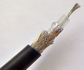
In electrical engineering, a transmission line is a specialized cable or other structure designed to conduct electromagnetic waves in a contained manner. The term applies when the conductors are long enough that the wave nature of the transmission must be taken into account. This applies especially to radio-frequency engineering because the short wavelengths mean that wave phenomena arise over very short distances. However, the theory of transmission lines was historically developed to explain phenomena on very long telegraph lines, especially submarine telegraph cables.
Chebyshev filters are analog or digital filters that have a steeper roll-off than Butterworth filters, and have either passband ripple or stopband ripple. Chebyshev filters have the property that they minimize the error between the idealized and the actual filter characteristic over the operating frequency range of the filter, but they achieve this with ripples in the passband. This type of filter is named after Pafnuty Chebyshev because its mathematical characteristics are derived from Chebyshev polynomials. Type I Chebyshev filters are usually referred to as "Chebyshev filters", while type II filters are usually called "inverse Chebyshev filters". Because of the passband ripple inherent in Chebyshev filters, filters with a smoother response in the passband but a more irregular response in the stopband are preferred for certain applications.

The Smith chart, is a graphical calculator or nomogram designed for electrical and electronics engineers specializing in radio frequency (RF) engineering to assist in solving problems with transmission lines and matching circuits.
Bosonic string theory is the original version of string theory, developed in the late 1960s and named after Satyendra Nath Bose. It is so called because it contains only bosons in the spectrum.
In physics, the Hamilton–Jacobi equation, named after William Rowan Hamilton and Carl Gustav Jacob Jacobi, is an alternative formulation of classical mechanics, equivalent to other formulations such as Newton's laws of motion, Lagrangian mechanics and Hamiltonian mechanics.
An elliptic filter is a signal processing filter with equalized ripple (equiripple) behavior in both the passband and the stopband. The amount of ripple in each band is independently adjustable, and no other filter of equal order can have a faster transition in gain between the passband and the stopband, for the given values of ripple. Alternatively, one may give up the ability to adjust independently the passband and stopband ripple, and instead design a filter which is maximally insensitive to component variations.

Oblate spheroidal coordinates are a three-dimensional orthogonal coordinate system that results from rotating the two-dimensional elliptic coordinate system about the non-focal axis of the ellipse, i.e., the symmetry axis that separates the foci. Thus, the two foci are transformed into a ring of radius in the x-y plane. Oblate spheroidal coordinates can also be considered as a limiting case of ellipsoidal coordinates in which the two largest semi-axes are equal in length.

The Π pad is a specific type of attenuator circuit in electronics whereby the topology of the circuit is formed in the shape of the Greek capital letter pi (Π).
Bilinear time–frequency distributions, or quadratic time–frequency distributions, arise in a sub-field of signal analysis and signal processing called time–frequency signal processing, and, in the statistical analysis of time series data. Such methods are used where one needs to deal with a situation where the frequency composition of a signal may be changing over time; this sub-field used to be called time–frequency signal analysis, and is now more often called time–frequency signal processing due to the progress in using these methods to a wide range of signal-processing problems.
Image impedance is a concept used in electronic network design and analysis and most especially in filter design. The term image impedance applies to the impedance seen looking into a port of a network. Usually a two-port network is implied but the concept can be extended to networks with more than two ports. The definition of image impedance for a two-port network is the impedance, Zi 1, seen looking into port 1 when port 2 is terminated with the image impedance, Zi 2, for port 2. In general, the image impedances of ports 1 and 2 will not be equal unless the network is symmetrical with respect to the ports.
Constant k filters, also k-type filters, are a type of electronic filter designed using the image method. They are the original and simplest filters produced by this methodology and consist of a ladder network of identical sections of passive components. Historically, they are the first filters that could approach the ideal filter frequency response to within any prescribed limit with the addition of a sufficient number of sections. However, they are rarely considered for a modern design, the principles behind them having been superseded by other methodologies which are more accurate in their prediction of filter response.
m-derived filters or m-type filters are a type of electronic filter designed using the image method. They were invented by Otto Zobel in the early 1920s. This filter type was originally intended for use with telephone multiplexing and was an improvement on the existing constant k type filter. The main problem being addressed was the need to achieve a better match of the filter into the terminating impedances. In general, all filters designed by the image method fail to give an exact match, but the m-type filter is a big improvement with suitable choice of the parameter m. The m-type filter section has a further advantage in that there is a rapid transition from the cut-off frequency of the passband to a pole of attenuation just inside the stopband. Despite these advantages, there is a drawback with m-type filters; at frequencies past the pole of attenuation, the response starts to rise again, and m-types have poor stopband rejection. For this reason, filters designed using m-type sections are often designed as composite filters with a mixture of k-type and m-type sections and different values of m at different points to get the optimum performance from both types.
A composite image filter is an electronic filter consisting of multiple image filter sections of two or more different types.

In general relativity, a point mass deflects a light ray with impact parameter by an angle approximately equal to

A signal travelling along an electrical transmission line will be partly, or wholly, reflected back in the opposite direction when the travelling signal encounters a discontinuity in the characteristic impedance of the line, or if the far end of the line is not terminated in its characteristic impedance. This can happen, for instance, if two lengths of dissimilar transmission lines are joined.

The T pad is a specific type of attenuator circuit in electronics whereby the topology of the circuit is formed in the shape of the letter "T".

The Peregrine soliton is an analytic solution of the nonlinear Schrödinger equation. This solution was proposed in 1983 by Howell Peregrine, researcher at the mathematics department of the University of Bristol.
Accelerations in special relativity (SR) follow, as in Newtonian Mechanics, by differentiation of velocity with respect to time. Because of the Lorentz transformation and time dilation, the concepts of time and distance become more complex, which also leads to more complex definitions of "acceleration". SR as the theory of flat Minkowski spacetime remains valid in the presence of accelerations, because general relativity (GR) is only required when there is curvature of spacetime caused by the energy–momentum tensor. However, since the amount of spacetime curvature is not particularly high on Earth or its vicinity, SR remains valid for most practical purposes, such as experiments in particle accelerators.
A proper reference frame in the theory of relativity is a particular form of accelerated reference frame, that is, a reference frame in which an accelerated observer can be considered as being at rest. It can describe phenomena in curved spacetime, as well as in "flat" Minkowski spacetime in which the spacetime curvature caused by the energy–momentum tensor can be disregarded. Since this article considers only flat spacetime—and uses the definition that special relativity is the theory of flat spacetime while general relativity is a theory of gravitation in terms of curved spacetime—it is consequently concerned with accelerated frames in special relativity.


