In numerical analysis, the condition number of a function measures how much the output value of the function can change for a small change in the input argument. This is used to measure how sensitive a function is to changes or errors in the input, and how much error in the output results from an error in the input. Very frequently, one is solving the inverse problem: given one is solving for x, and thus the condition number of the (local) inverse must be used.
In computational mathematics, an iterative method is a mathematical procedure that uses an initial value to generate a sequence of improving approximate solutions for a class of problems, in which the n-th approximation is derived from the previous ones.
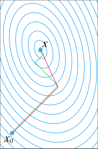
In numerical analysis, Newton's method, also known as the Newton–Raphson method, named after Isaac Newton and Joseph Raphson, is a root-finding algorithm which produces successively better approximations to the roots of a real-valued function. The most basic version starts with a real-valued function f, its derivative f′, and an initial guess x0 for a root of f. If f satisfies certain assumptions and the initial guess is close, then

Poisson's equation is an elliptic partial differential equation of broad utility in theoretical physics. For example, the solution to Poisson's equation is the potential field caused by a given electric charge or mass density distribution; with the potential field known, one can then calculate electrostatic or gravitational (force) field. It is a generalization of Laplace's equation, which is also frequently seen in physics. The equation is named after French mathematician and physicist Siméon Denis Poisson.
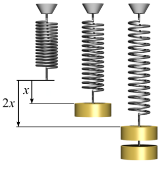
In physics, Hooke's law is an empirical law which states that the force needed to extend or compress a spring by some distance scales linearly with respect to that distance—that is, Fs = kx, where k is a constant factor characteristic of the spring, and x is small compared to the total possible deformation of the spring. The law is named after 17th-century British physicist Robert Hooke. He first stated the law in 1676 as a Latin anagram. He published the solution of his anagram in 1678 as: ut tensio, sic vis. Hooke states in the 1678 work that he was aware of the law since 1660.

The Drude model of electrical conduction was proposed in 1900 by Paul Drude to explain the transport properties of electrons in materials. Basically, Ohm's law was well established and stated that the current J and voltage V driving the current are related to the resistance R of the material. The inverse of the resistance is known as the conductance. When we consider a metal of unit length and unit cross sectional area, the conductance is known as the conductivity, which is the inverse of resistivity. The Drude model attempts to explain the resistivity of a conductor in terms of the scattering of electrons by the relatively immobile ions in the metal that act like obstructions to the flow of electrons.
In statistics, a studentized residual is the dimensionless ratio resulting from the division of a residual by an estimate of its standard deviation, both expressed in the same units. It is a form of a Student's t-statistic, with the estimate of error varying between points.
In plasmas and electrolytes, the Debye length, is a measure of a charge carrier's net electrostatic effect in a solution and how far its electrostatic effect persists. With each Debye length the charges are increasingly electrically screened and the electric potential decreases in magnitude by 1/e. A Debye sphere is a volume whose radius is the Debye length. Debye length is an important parameter in plasma physics, electrolytes, and colloids. The corresponding Debye screening wave vector for particles of density , charge at a temperature is given by in Gaussian units. Expressions in MKS units will be given below. The analogous quantities at very low temperatures are known as the Thomas–Fermi length and the Thomas–Fermi wave vector. They are of interest in describing the behaviour of electrons in metals at room temperature.
In mathematics, the conjugate gradient method is an algorithm for the numerical solution of particular systems of linear equations, namely those whose matrix is positive-definite. The conjugate gradient method is often implemented as an iterative algorithm, applicable to sparse systems that are too large to be handled by a direct implementation or other direct methods such as the Cholesky decomposition. Large sparse systems often arise when numerically solving partial differential equations or optimization problems.
In statistics, ordinary least squares (OLS) is a type of linear least squares method for choosing the unknown parameters in a linear regression model by the principle of least squares: minimizing the sum of the squares of the differences between the observed dependent variable in the input dataset and the output of the (linear) function of the independent variable.
Methods of computing square roots are algorithms for approximating the non-negative square root of a positive real number . Since all square roots of natural numbers, other than of perfect squares, are irrational, square roots can usually only be computed to some finite precision: these methods typically construct a series of increasingly accurate approximations.
In numerical linear algebra, the method of successive over-relaxation (SOR) is a variant of the Gauss–Seidel method for solving a linear system of equations, resulting in faster convergence. A similar method can be used for any slowly converging iterative process.
In statistics, generalized least squares (GLS) is a method used to estimate the unknown parameters in a linear regression model. It is used when there is a non-zero amount of correlation between the residuals in the regression model. GLS is employed to improve statistical efficiency and reduce the risk of drawing erroneous inferences, as compared to conventional least squares and weighted least squares methods. It was first described by Alexander Aitken in 1935.
In mathematics and economics, transportation theory or transport theory is a name given to the study of optimal transportation and allocation of resources. The problem was formalized by the French mathematician Gaspard Monge in 1781.
Equilibrium constants are determined in order to quantify chemical equilibria. When an equilibrium constant K is expressed as a concentration quotient,
The topic of heteroskedasticity-consistent (HC) standard errors arises in statistics and econometrics in the context of linear regression and time series analysis. These are also known as heteroskedasticity-robust standard errors, Eicker–Huber–White standard errors, to recognize the contributions of Friedhelm Eicker, Peter J. Huber, and Halbert White.
Tukey's range test, also known as Tukey's test, Tukey method, Tukey's honest significance test, or Tukey's HSDtest, is a single-step multiple comparison procedure and statistical test. It can be used to find means that are significantly different from each other.
The purpose of this page is to provide supplementary materials for the ordinary least squares article, reducing the load of the main article with mathematics and improving its accessibility, while at the same time retaining the completeness of exposition.
Linear least squares (LLS) is the least squares approximation of linear functions to data. It is a set of formulations for solving statistical problems involved in linear regression, including variants for ordinary (unweighted), weighted, and generalized (correlated) residuals. Numerical methods for linear least squares include inverting the matrix of the normal equations and orthogonal decomposition methods.
Numerical methods for linear least squares entails the numerical analysis of linear least squares problems.


