This article relies largely or entirely on a single source. Relevant discussion may be found on the talk page. Please help improve this article by introducing citations to additional sources.(December 2011)
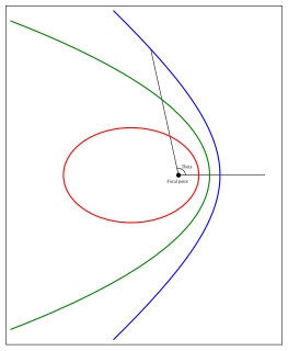
Orbital perturbation analysis is the activity of determining why a satellite's orbit differs from the mathematical ideal orbit. A satellite's orbit in an ideal two-body system describes a conic section, usually an ellipse. In reality, there are several factors that cause the conic section to continually change. These deviations from the ideal Kepler's orbit are called perturbations.
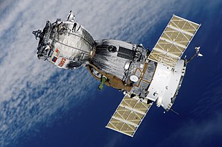
In the context of spaceflight, a satellite is an artificial object which has been intentionally placed into orbit. Such objects are sometimes called artificial satellites to distinguish them from natural satellites such as Earth's Moon.
In celestial mechanics, a Kepler orbit is the motion of one body relative to another, as an ellipse, parabola, or hyperbola, which forms a two-dimensional orbital plane in three-dimensional space. It considers only the point-like gravitational attraction of two bodies, neglecting perturbations due to gravitational interactions with other objects, atmospheric drag, solar radiation pressure, a non-spherical central body, and so on. It is thus said to be a solution of a special case of the two-body problem, known as the Kepler problem. As a theory in classical mechanics, it also does not take into account the effects of general relativity. Keplerian orbits can be parametrized into six orbital elements in various ways.
In astronomy, perturbation is the complex motion of a massive body subject to forces other than the gravitational attraction of a single other massive body. The other forces can include a third body, resistance, as from an atmosphere, and the off-center attraction of an oblate or otherwise misshapen body.
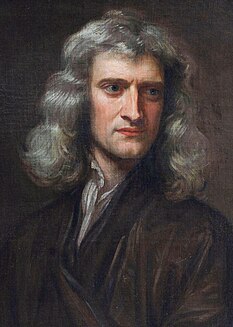
It has long been recognized that the Moon does not follow a perfect orbit, and many theories and models have been examined over the millennia to explain it. Isaac Newton determined the primary contributing factor to orbital perturbation of the moon was that the shape of the Earth is actually an oblate spheroid due to its spin, and he used the perturbations of the lunar orbit to estimate the oblateness of the Earth.[dubious–discuss][citation needed]
Lunar theory attempts to account for the motions of the Moon. There are many small variations in the Moon's motion, and many attempts have been made to account for them. After centuries of being problematic, lunar motion is now modeled to a very high degree of accuracy.
Sir Isaac Newton was an English mathematician, physicist, astronomer, theologian, and author who is widely recognised as one of the most influential scientists of all time, and a key figure in the scientific revolution. His book Philosophiæ Naturalis Principia Mathematica, first published in 1687, laid the foundations of classical mechanics. Newton also made seminal contributions to optics, and shares credit with Gottfried Wilhelm Leibniz for developing the infinitesimal calculus.
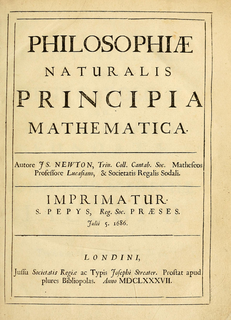
In Newton's Philosophiæ Naturalis Principia Mathematica, he demonstrated that the gravitational force between two mass points is inversely proportional to the square of the distance between the points, and he fully solved the corresponding "two-body problem" demonstrating that the radius vector between the two points would describe an ellipse. But no exact closed analytical form could be found for the three-body problem. Instead, mathematical models called "orbital perturbation analysis" have been developed. With these techniques a quite accurate mathematical description of the trajectories of all the planets could be obtained. Newton recognized that the Moon's perturbations could not entirely be accounted for using just the solution to the three-body problem, as the deviations from a pure Kepler orbit around the Earth are much larger than deviations of the orbits of the planets from their own Sun-centered Kepler orbits, caused by the gravitational attraction between the planets. With the availability of digital computers and the ease with which we can now compute orbits, this problem has partly disappeared, as the motion of all celestial bodies including planets, satellites, asteroids and comets can be modeled and predicted with almost perfect accuracy using the method of the numerical propagation of the trajectories. Nevertheless, several analytical closed form expressions for the effect of such additional "perturbing forces" are still very useful.
Philosophiæ Naturalis Principia Mathematica, often referred to as simply the Principia, is a work in three books by Isaac Newton, in Latin, first published 5 July 1687. After annotating and correcting his personal copy of the first edition, Newton published two further editions, in 1713 and 1726. The Principia states Newton's laws of motion, forming the foundation of classical mechanics; Newton's law of universal gravitation; and a derivation of Kepler's laws of planetary motion.
In physics and classical mechanics, the three-body problem is the problem of taking the initial positions and velocities of three point masses and solving for their subsequent motion according to Newton's laws of motion and Newton's law of universal gravitation. The three-body problem is a special case of the n-body problem. Unlike two-body problems, no closed-form solution exists for all sets of initial conditions, and numerical methods are generally required.
The precise modeling of the motion of the Moon has been a difficult task. The best and most accurate modeling for the lunar orbit before the availability of digital computers was obtained with the complicated Delaunay and Brown's lunar theories.
Charles-Eugène Delaunay was a French astronomer and mathematician. His lunar motion studies were important in advancing both the theory of planetary motion and mathematics.
Ernest William Brown FRS was an English mathematician and astronomer, who spent the majority of his career working in the United States and became a naturalised American citizen in 1923.
In general
All celestial bodies of the Solar System follow in first approximation a Kepler orbit around a central body. For a satellite (artificial or natural) this central body is a planet. But both due to gravitational forces caused by the Sun and other celestial bodies and due to the flattening of its planet (caused by its rotation which makes the planet slightly oblate and therefore the result of the Shell theorem not fully applicable) the satellite will follow an orbit around the Earth that deviates more than the Kepler orbits observed for the planets.
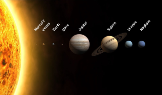
The Solar System is the gravitationally bound planetary system of the Sun and the objects that orbit it, either directly or indirectly. Of the objects that orbit the Sun directly, the largest are the eight planets, with the remainder being smaller objects, such as the five dwarf planets and small Solar System bodies. Of the objects that orbit the Sun indirectly—the moons—two are larger than the smallest planet, Mercury.
In classical mechanics, the shell theorem gives gravitational simplifications that can be applied to objects inside or outside a spherically symmetrical body. This theorem has particular application to astronomy.
Perturbation of spacecraft orbits
For man-made spacecraft orbiting the Earth at comparatively low altitudes the deviations from a Kepler orbit are much larger than for the Moon. The approximation of the gravitational force of the Earth to be that of a homogeneous sphere gets worse the closer one gets to the Earth surface and the majority of the artificial Earth satellites are in orbits that are only a few hundred kilometers over the Earth surface. Furthermore, they are (as opposed to the Moon) significantly affected by the solar radiation pressure because of their large cross-section-to-mass ratio; this applies in particular to 3-axis stabilized spacecraft with large solar arrays and is allowed for in calculation of graveyard orbits. In addition they are significantly affected by rarefied air below 800–1000km. The air drag at high altitudes is also dependent on solar activity.
A graveyard orbit, also called a junk orbit or disposal orbit, is an orbit that lies away from common operational orbits. One significant graveyard orbit is a supersynchronous orbit well above geosynchronous orbit. Satellites are typically moved into such orbits at the end of their operational life to reduce the probability of colliding with operational spacecraft and generating space debris.
Space weather is a branch of space physics and aeronomy, or heliophysics, concerned with the time varying conditions within the Solar System, including the solar wind, emphasizing the space surrounding the Earth, including conditions in the magnetosphere, ionosphere, thermosphere, and exosphere. Space weather is distinct from but conceptually related to the terrestrial weather of the atmosphere of Earth. The term space weather was first used in the 1950s and came into common usage in the 1990s..
Mathematical approach
Consider any function
of the position
and the velocity
From the chain rule of differentiation one gets that the time derivative of is
where are the components of the force per unit mass acting on the body.
If now is a "constant of motion" for a Kepler orbit like for example an orbital element and the force is corresponding "Kepler force"
one has that .
If the force is the sum of the "Kepler force" and an additional force (force per unit mass)
i.e.
one therefore has
and that the change of in the time from to is
If now the additional force is sufficiently small that the motion will be close to that of a Kepler orbit one gets an approximate value for by evaluating this integral assuming to precisely follow this Kepler orbit.
In general one wants to find an approximate expression for the change over one orbital revolution using the true anomaly as integration variable, i.e. as
(1)
This integral is evaluated setting , the elliptical Kepler orbit in polar angles. For the transformation of integration variable from time to true anomaly it was used that the angular momentum by definition of the parameter for a Kepler orbit (see equation (13) of the Kepler orbit article).
For the special case where the Kepler orbit is circular or almost circular
If is the perturbing force and is the velocity vector of the Kepler orbit the equation (1) takes the form:
(3)
and for a circular or almost circular orbit
(4)
From the change of the parameter the new semi-major axis and the new period are computed (relations (43) and (44) of the Kepler orbit article).
Perturbation of the orbital plane
Let and make up a rectangular coordinate system in the plane of the reference Kepler orbit. If is the argument of perigee relative the and coordinate system the true anomaly is given by and the approximate change of the orbital pole (defined as the unit vector in the direction of the angular momentum) is
(5)
where is the component of the perturbing force in the direction, is the velocity component of the Kepler orbit orthogonal to radius vector and is the distance to the center of the Earth.
For a circular or almost circular orbit (5) simplifies to
(6)
Example
In a circular orbit a low-force propulsion system (Ion thruster) generates a thrust (force per unit mass) of in the direction of the orbital pole in the half of the orbit for which is positive and in the opposite direction in the other half. The resulting change of orbit pole after one orbital revolution of duration is
(7)
The average change rate is therefore
(8)
where is the orbital velocity in the circular Kepler orbit.
Perturbation of the eccentricity vector
Rather than applying (1) and (2) on the partial derivatives of the orbital elements eccentricity and argument of perigee directly one should apply these relations for the eccentricity vector. First of all the typical application is a near-circular orbit. But there are also mathematical advantages working with the partial derivatives of the components of this vector also for orbits with a significant eccentricity.
Equations (60), (55) and (52) of the Kepler orbit article say that the eccentricity vector is
(9)
where
(10)
(11)
from which follows that
(12)
(13)
where
(14)
(15)
(Equations (18) and (19) of the Kepler orbit article)
The eccentricity vector is by definition always in the osculating orbital plane spanned by and and formally there is also a derivative
with
corresponding to the rotation of the orbital plane
But in practice the in-plane change of the eccentricity vector is computed as
(16)
ignoring the out-of-plane force and the new eccentricity vector
is subsequently projected to the new orbital plane orthogonal to the new orbit normal
computed as described above.
Example
The Sun is in the orbital plane of a spacecraft in a circular orbit with radius and consequently with a constant orbital velocity . If and make up a rectangular coordinate system in the orbital plane such that points to the Sun and assuming that the solar radiation pressure force per unit mass is constant one gets that
where is the polar angle of in the , system. Applying (2) one gets that
(17)
This means the eccentricity vector will gradually increase in the direction orthogonal to the Sun direction. This is true for any orbit with a small eccentricity, the direction of the small eccentricity vector does not matter. As is the orbital period this means that the average rate of this increase will be
The effect of the Earth flattening
Figure 1: The unit vectors
In the article Geopotential model the modeling of the gravitational field as a sum of spherical harmonics is discussed. By far, the dominating term is the "J2-term". This is a "zonal term" and corresponding force is therefore completely in a longitudinal plane with one component in the radial direction and one component with the unit vector orthogonal to the radial direction towards north. These directions and are illustrated in Figure 1.
Figure 2: The unit vector orthogonal to in the direction of motion and the orbital pole . The force component is marked as "F"
To be able to apply relations derived in the previous section the force component must be split into two orthogonal components and as illustrated in figure 2
Let make up a rectangular coordinate system with origin in the center of the Earth (in the center of the Reference ellipsoid) such that points in the direction north and such that are in the equatorial plane of the Earth with pointing towards the ascending node, i.e. towards the blue point of Figure 2.
The components of the unit vectors
making up the local coordinate system (of which are illustrated in figure 2) relative the are
where is the polar argument of relative the orthogonal unit vectors and in the orbital plane
Firstly
where is the angle between the equator plane and (between the green points of figure 2) and from equation (12) of the article Geopotential model one therefore gets that
(18)
Secondly the projection of direction north, , on the plane spanned by is
and this projection is
where is the unit vector orthogonal to the radial direction towards north illustrated in figure 1.
From equation (12) of the article Geopotential model one therefore gets that
where is the eccentricity and is the argument of perigee of the reference Kepler orbit
As all integrals of type
are zero if not both and are even one gets from (21) that
As
this can be written
(22)
As is an inertially fixed vector (the direction of the spin axis of the Earth) relation (22) is the equation of motion for a unit vector describing a cone around with a precession rate (radians per orbit) of
In terms of orbital elements this is expressed as
(23)
(24)
where
is the inclination of the orbit to the equatorial plane of the Earth
is the right ascension of the ascending node
Perturbation of the eccentricity vector
From (16), (18) and (19) follows that in-plane perturbation of the eccentricity vector is
(25)
the new eccentricity vector being the projection of
are the components of the eccentricity vector in the coordinate system this integral (25) can be evaluated analytically, the result is
(26)
This the difference equation of motion for the eccentricity vector to form a circle, the magnitude of the eccentricity staying constant.
Translating this to orbital elements it must be remembered that the new eccentricity vector obtained by adding to the old must be projected to the new orbital plane obtained by applying (23) and (24)
Figure 3: The change in "argument of perigee" after one orbit is the sum of a contribution caused by the in-plane force components and a contribution caused by the use of the ascending node as reference
This is illustrated in figure 3:
To the change in argument of the eccentricity vector
must be added an increment due to the precession of the orbital plane (caused by the out-of-plane force component) amounting to
One therefore gets that
(27)
(28)
In terms of the components of the eccentricity vector relative the coordinate system that precesses around the polar axis of the Earth the same is expressed as follows
(29)
where the first term is the in-plane perturbation of the eccentricity vector and the second is the effect of the new position of the ascending node in the new plane
From (28) follows that is zero if . This fact is used for Molniya orbits having an inclination of 63.4 deg. An orbit with an inclination of 180 - 63.4 deg = 116.6 deg would in the same way have a constant argument of perigee.
Proof
Proof that the integral
(30)
where:
has the value
(31)
Integrating the first term of the integrand one gets:
(32)
and
(33)
For the second term one gets:
(34)
and
(35)
For the third term one gets:
(36)
and
(37)
For the fourth term one gets:
(38)
and
(39)
Adding the right hand sides of (32), (34), (36) and (38) one gets
Adding the right hand sides of (33), (35), (37) and (39) one gets
Related Research Articles
In astronomy, Kepler's laws of planetary motion are three scientific laws describing the motion of planets around the Sun.
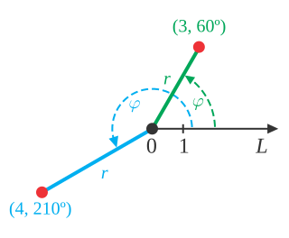
In mathematics, the polar coordinate system is a two-dimensional coordinate system in which each point on a plane is determined by a distance from a reference point and an angle from a reference direction.
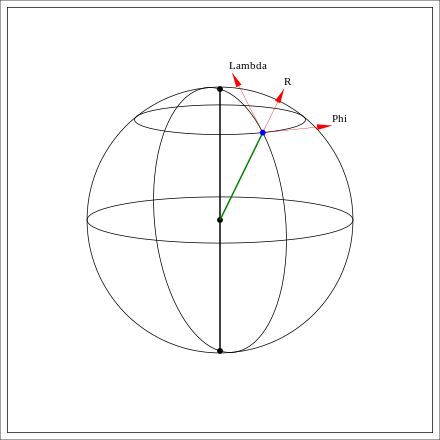
In mathematics, a spherical coordinate system is a coordinate system for three-dimensional space where the position of a point is specified by three numbers: the radial distance of that point from a fixed origin, its polar angle measured from a fixed zenith direction, and the azimuth angle of its orthogonal projection on a reference plane that passes through the origin and is orthogonal to the zenith, measured from a fixed reference direction on that plane. It can be seen as the three-dimensional version of the polar coordinate system.
In mathematics, a Fourier series is a periodic function composed of harmonically related sinusoids, combined by a weighted summation. With appropriate weights, one cycle of the summation can be made to approximate an arbitrary function in that interval. As such, the summation is a synthesis of another function. The discrete-time Fourier transform is an example of synthesis. The process of deriving the weights that describe a given function is a form of Fourier analysis. For functions on unbounded intervals, the analysis and synthesis analogies are Fourier transform and inverse transform.
In calculus, and more generally in mathematical analysis, integration by parts or partial integration is a process that finds the integral of a product of functions in terms of the integral of their derivative and antiderivative. It is frequently used to transform the antiderivative of a product of functions into an antiderivative for which a solution can be more easily found. The rule can be readily derived by integrating the product rule of differentiation.
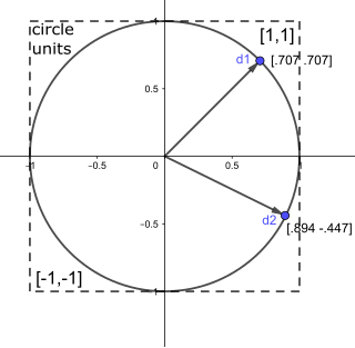
In mathematics, a unit vector in a normed vector space is a vector of length 1. A unit vector is often denoted by a lowercase letter with a circumflex, or "hat": . The term direction vector is used to describe a unit vector being used to represent spatial direction, and such quantities are commonly denoted as d. Two 2D direction vectors, d1 and d2 are illustrated. 2D spatial directions represented this way are numerically equivalent to points on the unit circle.
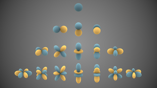
In mathematics and physical science, spherical harmonics are special functions defined on the surface of a sphere. They are often employed in solving partial differential equations that commonly occur in science. The spherical harmonics are a complete set of orthogonal functions on the sphere, and thus may be used to represent functions defined on the surface of a sphere, just as circular functions are used to represent functions on a circle via Fourier series. Like the sines and cosines in Fourier series, the spherical harmonics may be organized by (spatial) angular frequency, as seen in the rows of functions in the illustration on the right. Further, spherical harmonics are basis functions for SO(3), the group of rotations in three dimensions, and thus play a central role in the group theoretic discussion of SO(3).
In mathematics, Pappus's centroid theorem is either of two related theorems dealing with the surface areas and volumes of surfaces and solids of revolution.
In classical mechanics, the Laplace–Runge–Lenz (LRL) vector is a vector used chiefly to describe the shape and orientation of the orbit of one astronomical body around another, such as a planet revolving around a star. For two bodies interacting by Newtonian gravity, the LRL vector is a constant of motion, meaning that it is the same no matter where it is calculated on the orbit; equivalently, the LRL vector is said to be conserved. More generally, the LRL vector is conserved in all problems in which two bodies interact by a central force that varies as the inverse square of the distance between them; such problems are called Kepler problems.
In celestial mechanics, true anomaly is an angular parameter that defines the position of a body moving along a Keplerian orbit. It is the angle between the direction of periapsis and the current position of the body, as seen from the main focus of the ellipse.
In astrodynamics or celestial mechanics, an elliptic orbit or elliptical orbit is a Kepler orbit with an eccentricity of less than 1; this includes the special case of a circular orbit, with eccentricity equal to 0. In a stricter sense, it is a Kepler orbit with the eccentricity greater than 0 and less than 1. In a wider sense, it is a Kepler orbit with negative energy. This includes the radial elliptic orbit, with eccentricity equal to 1.
The rigid rotor is a mechanical model of rotating systems. An arbitrary rigid rotor is a 3-dimensional rigid object, such as a top. To orient such an object in space requires three angles, known as Euler angles. A special rigid rotor is the linear rotor requiring only two angles to describe, for example of a diatomic molecule. More general molecules are 3-dimensional, such as water, ammonia, or methane.
In calculus, Leibniz's rule for differentiation under the integral sign, named after Gottfried Leibniz, states that for an integral of the form
A parametric surface is a surface in the Euclidean space which is defined by a parametric equation with two parameters Parametric representation is a very general way to specify a surface, as well as implicit representation. Surfaces that occur in two of the main theorems of vector calculus, Stokes' theorem and the divergence theorem, are frequently given in a parametric form. The curvature and arc length of curves on the surface, surface area, differential geometric invariants such as the first and second fundamental forms, Gaussian, mean, and principal curvatures can all be computed from a given parametrization.
Photon polarization is the quantum mechanical description of the classical polarized sinusoidal plane electromagnetic wave. An individual photon can be described as having right or left circular polarization, or a superposition of the two. Equivalently, a photon can be described as having horizontal or vertical linear polarization, or a superposition of the two.
In fluid dynamics, the Oseen equations describe the flow of a viscous and incompressible fluid at small Reynolds numbers, as formulated by Carl Wilhelm Oseen in 1910. Oseen flow is an improved description of these flows, as compared to Stokes flow, with the (partial) inclusion of convective acceleration.
The direct-quadrature-zerotransformation or zero-direct-quadraturetransformation is a tensor that rotates the reference frame of a three-element vector or a three-by-three element matrix in an effort to simplify analysis. The DQZ transform is the product of the Clarke transform and the Park transform, first proposed in 1929 by Robert H. Park.
In classical mechanics, the central-force problem is to determine the motion of a particle under the influence of a single central force. A central force is a force that points from the particle directly towards a fixed point in space, the center, and whose magnitude only depends on the distance of the object to the center. In many important cases, the problem can be solved analytically, i.e., in terms of well-studied functions such as trigonometric functions.
In orbital mechanics, a frozen orbit is an orbit for an artificial satellite in which natural drifting due to the central body's shape has been minimized by careful selection of the orbital parameters. Typically, this is an orbit in which, over a long period of time, the satellite's altitude remains constant at the same point in each orbit. Changes in the inclination, position of the lowest point of the orbit, and eccentricity have been minimized by choosing initial values so that their perturbations cancel out. This results in a long-term stable orbit that minimizes the use of station-keeping propellant.
This page is based on this Wikipedia article Text is available under the CC BY-SA 4.0 license; additional terms may apply. Images, videos and audio are available under their respective licenses.