Powell's method

Last updated November 05, 2022

Powell's method, strictly Powell's conjugate direction method, is an algorithm proposed by Michael J. D. Powell for finding a local minimum of a function. The function need not be differentiable, and no derivatives are taken.

The function must be a real-valued function of a fixed number of real-valued inputs. The caller passes in the initial point. The caller also passes in a set of initial search vectors. Typically N search vectors (say ${\textstyle \{s_{1},\dots ,s_{N}\}}$ ) are passed in which are simply the normals aligned to each axis.^[1]

The method minimises the function by a bi-directional search along each search vector, in turn. The bi-directional line search along each search vector can be done by Golden-section search or Brent's method. Let the minima found during each bi-directional line search be ${\textstyle \{x_{0}+\alpha _{1}s_{1},{x}_{0}+\sum _{i=1}^{2}\alpha _{i}{s}_{i},\dots ,{x}_{0}+\sum _{i=1}^{N}\alpha _{i}{s}_{i}\}}$ , where ${\textstyle {x}_{0}}$ is the initial starting point and ${\textstyle \alpha _{i}}$ is the scalar determined during bi-directional search along ${\textstyle {s}_{i}}$ . The new position ( ${\textstyle x_{1}}$ ) can then be expressed as a linear combination of the search vectors i.e. ${\textstyle x_{1}=x_{0}+\sum _{i=1}^{N}\alpha _{i}s_{i}}$ . The new displacement vector ( ${\textstyle \sum _{i=1}^{N}\alpha _{i}s_{i}}$ ) becomes a new search vector, and is added to the end of the search vector list. Meanwhile, the search vector which contributed most to the new direction, i.e. the one which was most successful ( ${\textstyle i_{d}=\arg \max _{i=1}^{N}|\alpha _{i}|\|s_{i}\|}$ ), is deleted from the search vector list. The new set of N search vectors is ${\textstyle \{s_{1},\dots ,s_{i_{d}-1},s_{i_{d}+1},\dots ,s_{N},\sum _{i=1}^{N}\alpha _{i}s_{i}\}}$ . The algorithm iterates an arbitrary number of times until no significant improvement is made.^[1]

The method is useful for calculating the local minimum of a continuous but complex function, especially one without an underlying mathematical definition, because it is not necessary to take derivatives. The basic algorithm is simple; the complexity is in the linear searches along the search vectors, which can be achieved via Brent's method.

Related Research Articles

<span class="mw-page-title-main">Gradient</span> Multivariate derivative (mathematics)

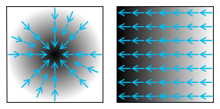
In vector calculus, the gradient of a scalar-valued differentiable function $f$ of several variables is the vector field $whose value at a point is the vector whose components are the partial derivatives of at . That is, for, its gradient is defined at the point in n- dimensional space as the vector$

In numerical analysis, Newton's method, also known as the Newton–Raphson method, named after Isaac Newton and Joseph Raphson, is a root-finding algorithm which produces successively better approximations to the roots of a real-valued function. The most basic version starts with a single-variable function $f$ defined for a real variable $x$ , the function's derivative $f'$ , and an initial guess $x 0$ for a root of $f$ . If the function satisfies sufficient assumptions and the initial guess is close, then

In mathematics, a power series is an infinite series of the form

In mathematics, differential forms provide a unified approach to define integrands over curves, surfaces, solids, and higher-dimensional manifolds. The modern notion of differential forms was pioneered by Élie Cartan. It has many applications, especially in geometry, topology and physics.

In mathematics, the Hodge star operator or Hodge star is a linear map defined on the exterior algebra of a finite-dimensional oriented vector space endowed with a nondegenerate symmetric bilinear form. Applying the operator to an element of the algebra produces the Hodge dual of the element. This map was introduced by W. V. D. Hodge.

In mathematics, a linear differential equation is a differential equation that is defined by a linear polynomial in the unknown function and its derivatives, that is an equation of the form

In mathematics, the directional derivative of a multivariable differentiable (scalar) function along a given vector v at a given point x intuitively represents the instantaneous rate of change of the function, moving through x with a velocity specified by v.

The Gauss–Newton algorithm is used to solve non-linear least squares problems, which is equivalent to minimizing a sum of squared function values. It is an extension of Newton's method for finding a minimum of a non-linear function. Since a sum of squares must be nonnegative, the algorithm can be viewed as using Newton's method to iteratively approximate zeroes of the sum, and thus minimizing the sum. It has the advantage that second derivatives, which can be challenging to compute, are not required.

In differential geometry of curves, the osculating circle of a sufficiently smooth plane curve at a given point p on the curve has been traditionally defined as the circle passing through p and a pair of additional points on the curve infinitesimally close to p. Its center lies on the inner normal line, and its curvature defines the curvature of the given curve at that point. This circle, which is the one among all tangent circles at the given point that approaches the curve most tightly, was named circulus osculans by Leibniz.

In mathematics, a differentiable manifold is a type of manifold that is locally similar enough to a vector space to allow one to apply calculus. Any manifold can be described by a collection of charts (atlas). One may then apply ideas from calculus while working within the individual charts, since each chart lies within a vector space to which the usual rules of calculus apply. If the charts are suitably compatible, then computations done in one chart are valid in any other differentiable chart.

In mathematics, the derivative is a fundamental construction of differential calculus and admits many possible generalizations within the fields of mathematical analysis, combinatorics, algebra, geometry, etc.

The softmax function, also known as softargmax or normalized exponential function, converts a vector of $K$ real numbers into a probability distribution of $K$ possible outcomes. It is a generalization of the logistic function to multiple dimensions, and used in multinomial logistic regression. The softmax function is often used as the last activation function of a neural network to normalize the output of a network to a probability distribution over predicted output classes, based on Luce's choice axiom.

In applied mathematics, polyharmonic splines are used for function approximation and data interpolation. They are very useful for interpolating and fitting scattered data in many dimensions. Special cases include thin plate splines and natural cubic splines in one dimension.

Covariance matrix adaptation evolution strategy (CMA-ES) is a particular kind of strategy for numerical optimization. Evolution strategies (ES) are stochastic, derivative-free methods for numerical optimization of non-linear or non-convex continuous optimization problems. They belong to the class of evolutionary algorithms and evolutionary computation. An evolutionary algorithm is broadly based on the principle of biological evolution, namely the repeated interplay of variation and selection: in each generation (iteration) new individuals are generated by variation, usually in a stochastic way, of the current parental individuals. Then, some individuals are selected to become the parents in the next generation based on their fitness or objective function value $. Like this, over the generation sequence, individuals with better and better -values are generated.$

Stochastic approximation methods are a family of iterative methods typically used for root-finding problems or for optimization problems. The recursive update rules of stochastic approximation methods can be used, among other things, for solving linear systems when the collected data is corrupted by noise, or for approximating extreme values of functions which cannot be computed directly, but only estimated via noisy observations.

In numerical optimization, the nonlinear conjugate gradient method generalizes the conjugate gradient method to nonlinear optimization. For a quadratic function

In mathematics and statistics, a circular mean or angular mean is a mean designed for angles and similar cyclic quantities, such as daytimes, and fractional parts of real numbers. This is necessary since most of the usual means may not be appropriate on angle-like quantities. For example, the arithmetic mean of 0° and 360° is 180°, which is misleading because 360° equals 0° modulo a full cycle. As another example, the "average time" between 11 PM and 1 AM is either midnight or noon, depending on whether the two times are part of a single night or part of a single calendar day. The circular mean is one of the simplest examples of circular statistics and of statistics of non-Euclidean spaces. This computation produces a different result than the arithmetic mean, with the difference being greater when the angles are widely distributed. For example, the arithmetic mean of the three angles 0°, 0° and 90° is (0+0+90)/3 = 30°, but the vector mean is 26.565°. Moreover, with the arithmetic mean the circular variance is only defined ±180°.

Non-linear least squares is the form of least squares analysis used to fit a set of m observations with a model that is non-linear in n unknown parameters (m ≥ n). It is used in some forms of nonlinear regression. The basis of the method is to approximate the model by a linear one and to refine the parameters by successive iterations. There are many similarities to linear least squares, but also some significant differences. In economic theory, the non-linear least squares method is applied in (i) the probit regression, (ii) threshold regression, (iii) smooth regression, (iv) logistic link regression, (v) Box-Cox transformed regressors.

<span class="mw-page-title-main">Logit-normal distribution</span>

In probability theory, a logit-normal distribution is a probability distribution of a random variable whose logit has a normal distribution. If Y is a random variable with a normal distribution, and P is the standard logistic function, then X = P(Y) has a logit-normal distribution; likewise, if X is logit-normally distributed, then Y = logit(X)= log is normally distributed. It is also known as the logistic normal distribution, which often refers to a multinomial logit version (e.g.).

In machine learning, Manifold regularization is a technique for using the shape of a dataset to constrain the functions that should be learned on that dataset. In many machine learning problems, the data to be learned do not cover the entire input space. For example, a facial recognition system may not need to classify any possible image, but only the subset of images that contain faces. The technique of manifold learning assumes that the relevant subset of data comes from a manifold, a mathematical structure with useful properties. The technique also assumes that the function to be learned is smooth: data with different labels are not likely to be close together, and so the labeling function should not change quickly in areas where there are likely to be many data points. Because of this assumption, a manifold regularization algorithm can use unlabeled data to inform where the learned function is allowed to change quickly and where it is not, using an extension of the technique of Tikhonov regularization. Manifold regularization algorithms can extend supervised learning algorithms in semi-supervised learning and transductive learning settings, where unlabeled data are available. The technique has been used for applications including medical imaging, geographical imaging, and object recognition.

References

1 2 Mathews, John H. "Module for Powell Search Method for a Minimum". California State University, Fullerton. Retrieved 16 June 2017.

Powell, M. J. D. (1964). "An efficient method for finding the minimum of a function of several variables without calculating derivatives". Computer Journal. 7 (2): 155–162. doi:10.1093/comjnl/7.2.155. hdl: 10338.dmlcz/103029 .
Press, WH; Teukolsky, SA; Vetterling, WT; Flannery, BP (2007). "Section 10.7. Direction Set (Powell's) Methods in Multidimensions". Numerical Recipes: The Art of Scientific Computing (3rd ed.). New York: Cambridge University Press. ISBN 978-0-521-88068-8.
Brent, Richard P. (1973). "Section 7.3: Powell's algorithm". Algorithms for minimization without derivatives. Englewood Cliffs, N.J.: Prentice-Hall. ISBN 0-486-41998-3.

This page is based on this Wikipedia article
Text is available under the CC BY-SA 4.0 license; additional terms may apply.
Images, videos and audio are available under their respective licenses.

[mathews-1] 1 2 Mathews, John H. "Module for Powell Search Method for a Minimum". California State University, Fullerton. Retrieved 16 June 2017.

[1]