The soil moisture velocity equation[1] describes the speed that water moves vertically through a soil under the combined actions of gravity and capillarity, a process known as infiltration. The equation is another form of the Richardson/Richards' equation.[2][3] The key difference being that the dependent variable is the position of the wetting front , which is a function of time, the water content and media properties. The soil moisture velocity equation consists of two terms. The first "advection-like" term was developed to simulate surface infiltration [4] and was extended to the water table[5], which was verified using data collected in a column experimental that was patterned after the famous experiment by Childs & Poulovassilis (1962)[6] and against exact solutions.[7][1]
The soil moisture velocity equation[1] or SMVE is an alternative interpretation of the Richards equation wherein the dependent variable is the position z of a wetting front of a particular moisture content with time.
where:
is the vertical coordinate [L] (positive downward),
The first term on the right-hand side of the SMVE is called the "advection-like" term, while the second term is called the "diffusion-like" term. The advection-like term of the Soil Moisture Velocity Equation is particularly useful for calculating the advance of wetting fronts for a liquid invading an unsaturated porous medium under the combined action of gravity and capillarity because it is convertible to an ordinary differential equation by neglecting the diffusion-like term.[5] and it avoids the problem of representative elementary volume by use of a fine water-content discretization and solution method.
This equation was converted into a set of three ordinary differential equations (ODEs)[5] using the method of lines[8] to convert the partial derivatives on the right-hand side of the equation into appropriate finite difference forms. These three ODEs represent the dynamics of infiltrating water, falling slugs, and capillary groundwater, respectively.
Derivation
This derivation of the 1-D soil moisture velocity equation[1] for calculating vertical flux of water in the vadose zone starts with conservation of mass for an unsaturated porous medium without sources or sinks:
We next insert the unsaturated Buckingham–Darcy flux:[9]
yielding Richards' equation[2] in mixed form because it includes both the water content and capillary head :
.
Applying the chain rule of differentiation to the right-hand side of Richards' equation:
.
Assuming that the constitutive relations for unsaturated hydraulic conductivity and soil capillarity are solely functions of the water content, and , respectively:
.
This equation implicitly defines a function that describes the position of a particular moisture content within the soil using a finite moisture-content discretization. Employing the Implicit function theorem, which by the cyclic rule required dividing both sides of this equation by to perform the change in variable, resulting in:
,
which can be written as:
.
Inserting the definition of the soil water diffusivity:
into the previous equation produces:
If we consider the velocity of a particular water content , then we can write the equation in the form of the Soil Moisture Velocity Equation:
Where D(θ) [L2/T] is 'the soil water diffusivity' as previously defined.
Note that with as the dependent variable, physical interpretation is difficult because all the factors that affect the divergence of the flux are wrapped up in the soil moisture diffusivity term . However, in the SMVE, the three factors that drive flow are in separate terms that have physical significance.
The primary assumptions used in the derivation of the Soil Moisture Velocity Equation are that and are not overly restrictive. Analytical and experimental results show that these assumptions are acceptable under most conditions in natural soils. In this case, the Soil Moisture Velocity Equation is equivalent to the 1-D Richards' equation, albeit with a change in dependent variable. This change of dependent variable is convenient because it reduces the complexity of the problem because compared to Richards' equation, which requires the calculation of the divergence of the flux, the SMVE represents a flux calculation, not a divergence calculation. The first term on the right-hand side of the SMVE represents the two scalar drivers of flow, gravity and the integrated capillarity of the wetting front. Considering just that term, the SMVE becomes:
where is the capillary head gradient that is driving the flux and the remaining conductivity term represents the ability of gravity to conduct flux through the soil. This term is responsible for the true advection of water through the soil under the combined influences of gravity and capillarity. As such, it is called the "advection-like" term.
Neglecting gravity and the scalar wetting front capillarity, we can consider only the second term on the right-hand side of the SMVE. In this case the Soil Moisture Velocity Equation becomes:
This term is strikingly similar to Fick's second law of diffusion. For this reason, this term is called the "diffusion-like" term of the SMVE.
This term represents the flux due to the shape of the wetting front , divided by the spatial gradient of the capillary head . Looking at this diffusion-like term, it is reasonable to ask when might this term be negligible? The first answer is that this term will be zero when the first derivative , because the second derivative will equal zero. One example where this occurs is in the case of an equilibrium hydrostatic moisture profile, when with z defined as positive upward. This is a physically realistic result because an equilibrium hydrostatic moisture profile is known to not produce fluxes.
Another instance when the diffusion-like term will be nearly zero is in the case of sharp wetting fronts, where the denominator of the diffusion-like term , causing the term to vanish. Notably, sharp wetting fronts are notoriously difficult to resolve and accurately solve with traditional numerical Richards' equation solvers.[11]
Finally, in the case of dry soils, tends towards , making the soil water diffusivity tend towards zero as well. In this case, the diffusion-like term would produce no flux.
Comparing against exact solutions of Richards' equation for infiltration into idealized soils developed by Ross & Parlange (1994)[12] revealed[1] that indeed, neglecting the diffusion-like term resulted in accuracy >99% in calculated cumulative infiltration. This result indicates that the advection-like term of the SMVE, converted into an ordinary differential equation using the method of lines, is an accurate ODE solution of the infiltration problem. This is consistent with the result published by Ogden et al.[5] who found errors in simulated cumulative infiltration of 0.3% using 263cm of tropical rainfall over an 8-month simulation to drive infiltration simulations that compared the advection-like SMVE solution against the numerical solution of Richards' equation.
Infiltration fronts in finite water-content domain
With reference to Figure 1, water infiltrating the land surface can flow through the pore space between and . Using the method of lines to convert the SMVE advection-like term into an ODE:
Given that any ponded depth of water on the land surface is , the Green and Ampt (1911)[13] assumption is employed,
represents the capillary head gradient that is driving the flow in the discretization or "bin". Therefore, the finite water-content equation in the case of infiltration fronts is:
Falling slugs
Falling slugs in the finite water-content domain. The water in each bin is considered a separate slug.
After rainfall stops and all surface water infiltrates, water in bins that contains infiltration fronts detaches from the land surface. Assuming that the capillarity at leading and trailing edges of this 'falling slug' of water is balanced, then the water falls through the media at the incremental conductivity associated with the bin:
.
This approach to solving the capillary-free solution is very similar to the kinematic wave approximation.
Capillary groundwater fronts
Groundwater capillary fronts in finite water-content domain
In this case, the flux of water to the bin occurs between bin j and i. Therefore, in the context of the method of lines:
and
which yields:
Note the "-1" in parentheses, representing the fact that gravity and capillarity are acting in opposite directions. The performance of this equation was verified,[7] using a column experiment fashioned after that by Childs and Poulovassilis (1962).[6] Results of that validation showed that the finite water-content vadose zone flux calculation method performed comparably to the numerical solution of Richards' equation. The photo shows apparatus. Data from this column experiment are available by clicking on this hot-linked DOI. These data are useful for evaluating models of near-surface water table dynamics.
It is noteworthy that the SMVE advection-like term solved using the finite moisture-content method completely avoids the need to estimate the specific yield. Calculating the specific yield as the water table nears the land surface is made cumbersome my non-linearities. However, the SMVE solved using a finite moisture-content discretization essentially does this automatically in the case of a dynamic near-surface water table.
Column experiment used to observe moisture response in a fine sand above a moving water table. Note stepper-motor controlled constant head reservoir (white bucket).
Notice and awards
The paper on the Soil Moisture Velocity Equation was highlighted by the editor in the issue of J. Adv. Modeling of Earth Systems when the paper was first published, and is in the public domain. The paper may be freely downloaded here by anyone. The paper describing the finite moisture-content solution of the advection-like term of the Soil Moisture Velocity Equation was selected to receive the 2015 Coolest Paper Award by the Early Career Hydrogeologists of the International Association of Hydrogeologists.
Related Research Articles
In mathematics, Laplace's equation is a second-order partial differential equation named after Pierre-Simon Laplace who first studied its properties. This is often written as
In physics, the Navier–Stokes equations, named after Claude-Louis Navier and George Gabriel Stokes, describe the motion of viscous fluid substances.
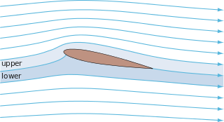
In fluid dynamics, potential flow describes the velocity field as the gradient of a scalar function: the velocity potential. As a result, a potential flow is characterized by an irrotational velocity field, which is a valid approximation for several applications. The irrotationality of a potential flow is due to the curl of the gradient of a scalar always being equal to zero.
In the field of physics, engineering, and earth sciences, advection is the transport of a substance or quantity by bulk motion. The properties of that substance are carried with it. Generally the majority of the advected substance is a fluid. The properties that are carried with the advected substance are conserved properties such as energy. An example of advection is the transport of pollutants or silt in a river by bulk water flow downstream. Another commonly advected quantity is energy or enthalpy. Here the fluid may be any material that contains thermal energy, such as water or air. In general, any substance or conserved, extensive quantity can be advected by a fluid that can hold or contain the quantity or substance.
In 1851, George Gabriel Stokes derived an expression, now known as Stokes law, for the frictional force – also called drag force – exerted on spherical objects with very small Reynolds numbers in a viscous fluid. Stokes' law is derived by solving the Stokes flow limit for small Reynolds numbers of the Navier–Stokes equations.
A continuity equation in physics is an equation that describes the transport of some quantity. It is particularly simple and powerful when applied to a conserved quantity, but it can be generalized to apply to any extensive quantity. Since mass, energy, momentum, electric charge and other natural quantities are conserved under their respective appropriate conditions, a variety of physical phenomena may be described using continuity equations.
The Grad–Shafranov equation is the equilibrium equation in ideal magnetohydrodynamics (MHD) for a two dimensional plasma, for example the axisymmetric toroidal plasma in a tokamak. This equation takes the same form as the Hicks equation from fluid dynamics. This equation is a two-dimensional, nonlinear, elliptic partial differential equation obtained from the reduction of the ideal MHD equations to two dimensions, often for the case of toroidal axisymmetry. Taking as the cylindrical coordinates, the flux function is governed by the equation,
Infiltration is the process by which water on the ground surface enters the soil. It is commonly used in both hydrology and soil sciences. The infiltration capacity is defined as the maximum rate of infiltration. It is most often measured in meters per day but can also be measured in other units of distance over time if necessary. The infiltration capacity decreases as the soil moisture content of soils surface layers increases. If the precipitation rate exceeds the infiltration rate, runoff will usually occur unless there is some physical barrier.
In analytical mechanics, a branch of theoretical physics, Routhian mechanics is a hybrid formulation of Lagrangian mechanics and Hamiltonian mechanics developed by Edward John Routh. Correspondingly, the Routhian is the function which replaces both the Lagrangian and Hamiltonian functions.
Potential vorticity (PV) is seen as one of the important theoretical successes of modern meteorology. It is a simplified approach for understanding fluid motions in a rotating system such as the Earth's atmosphere and ocean. Its development traces back to the circulation theorem by Bjerknes in 1898, which is a specialized form of Kelvin's circulation theorem. Starting from Hoskins et al., 1985, PV has been more commonly used in operational weather diagnosis such as tracing dynamics of air parcels and inverting for the full flow field. Even after detailed numerical weather forecasts on finer scales were made possible by increases in computational power, the PV view is still used in academia and routine weather forecasts, shedding light on the synoptic scale features for forecasters and researchers.
The Richards equation represents the movement of water in unsaturated soils, and is attributed to Lorenzo A. Richards who published the equation in 1931. It is a nonlinear partial differential equation, which is often difficult to approximate since it does not have a closed-form analytical solution. Although attributed to Richards, it is established that this equation was actually discovered 9 years earlier by Lewis Fry Richardson in his book "Weather prediction by numerical process" published in 1922 (p.108).
The Gross–Pitaevskii equation describes the ground state of a quantum system of identical bosons using the Hartree–Fock approximation and the pseudopotential interaction model.
HydroGeoSphere (HGS) is a 3D control-volume finite element groundwater model, and is based on a rigorous conceptualization of the hydrologic system consisting of surface and subsurface flow regimes. The model is designed to take into account all key components of the hydrologic cycle. For each time step, the model solves surface and subsurface flow, solute and energy transport equations simultaneously, and provides a complete water and solute balance.
In fluid dynamics, the Oseen equations describe the flow of a viscous and incompressible fluid at small Reynolds numbers, as formulated by Carl Wilhelm Oseen in 1910. Oseen flow is an improved description of these flows, as compared to Stokes flow, with the (partial) inclusion of convective acceleration.
In fluid dynamics, the mild-slope equation describes the combined effects of diffraction and refraction for water waves propagating over bathymetry and due to lateral boundaries—like breakwaters and coastlines. It is an approximate model, deriving its name from being originally developed for wave propagation over mild slopes of the sea floor. The mild-slope equation is often used in coastal engineering to compute the wave-field changes near harbours and coasts.
In fluid dynamics, a cnoidal wave is a nonlinear and exact periodic wave solution of the Korteweg–de Vries equation. These solutions are in terms of the Jacobi elliptic function cn, which is why they are coined cnoidal waves. They are used to describe surface gravity waves of fairly long wavelength, as compared to the water depth.
In mathematics, potential flow around a circular cylinder is a classical solution for the flow of an inviscid, incompressible fluid around a cylinder that is transverse to the flow. Far from the cylinder, the flow is unidirectional and uniform. The flow has no vorticity and thus the velocity field is irrotational and can be modeled as a potential flow. Unlike a real fluid, this solution indicates a net zero drag on the body, a result known as d'Alembert's paradox.
Fluid motion can be said to be a two-dimensional flow when the flow velocity at every point is parallel to a fixed plane. The velocity at any point on a given normal to that fixed plane should be constant.
The finite water-content vadose zone flux method represents a one-dimensional alternative to the numerical solution of Richards' equation for simulating the movement of water in unsaturated soils. The finite water-content method solves the advection-like term of the Soil Moisture Velocity Equation, which is an ordinary differential equation alternative to the Richards partial differential equation. The Richards equation is difficult to approximate in general because it does not have a closed-form analytical solution except in a few cases. The finite water-content method, is perhaps the first generic replacement for the numerical solution of the Richards' equation. The finite water-content solution has several advantages over the Richards equation solution. First, as an ordinary differential equation it is explicit, guaranteed to converge and computationally inexpensive to solve. Second, using a finite volume solution methodology it is guaranteed to conserve mass. The finite water content method readily simulates sharp wetting fronts, something that the Richards solution struggles with. The main limiting assumption required to use the finite water-content method is that the soil be homogeneous in layers.
In fluid dynamics, Hicks equation or sometimes also referred as Bragg–Hawthorne equation or Squire–Long equation is a partial differential equation that describes the distribution of stream function for axisymmetric inviscid fluid, named after William Mitchinson Hicks, who derived it first in 1898. The equation was also re-derived by Stephen Bragg and William Hawthorne in 1950 and by Robert R. Long in 1953 and by Herbert Squire in 1956. The Hicks equation without swirl was first introduced by George Gabriel Stokes in 1842. The Grad–Shafranov equation appearing in plasma physics also takes the same form as the Hicks equation.
References
1 2 3 4 5 Ogden, F.L, M.B. Allen, W.Lai, J. Zhu, C.C. Douglas, M. Seo, and C.A. Talbot, 2017. The Soil Moisture Velocity Equation, J. Adv. Modeling Earth Syst.https://doi.org/10.1002/2017MS000931
↑ Richards, L. A. (1931), Capillary conduction of liquids through porous mediums, J. Appl. Phys., 1(5), 318–333.
↑ Talbot, C.A., and F. L. Ogden (2008), A method for computing infiltration and redistribution in a discretized moisture content domain, Water Resour. Res., 44(8), doi: 10.1029/2008WR006815.
1 2 3 4 Ogden, F. L., W. Lai, R. C. Steinke, J. Zhu, C. A. Talbot, and J. L. Wilson (2015), A new general 1-D vadose zone solution method, Water Resour.Res., 51, doi:10.1002/2015WR017126.
1 2 Childs, E. C., and A. Poulovassilis (1962), The moisture profile above a moving water table, Soil Sci. J., 13(2), 271–285.
1 2 Ogden, F. L., W. Lai, R. C. Steinke, and J. Zhu (2015b), Validation of finite water-content vadose zone dynamics method using column experiments with a moving water table and applied surface flux, Water Resour. Res., 10.1002/2014WR016454.
↑ Jury, W. A., and R. Horton, 2004. Soil physics. John Wiley & Sons.
↑ Philip, J.R., 1957. Theory of infiltration 1: The infiltration equation and its solution. Soil Sci. 83(5):345-357.
↑ Farthing, M. W., & Ogden, F. L. (2017). Numerical Solution of Richards’ Equation: A Review of Advances and Challenges. Soil Science Society of America J.
↑ Ross, P.J., and J.-Y. Parlange, 1994. Comparing exact and numerical solutions of Richards' for 1-dimensional infiltration and drainage, Soil Sci. 157(6):341-344.
↑ Green, W. H., and G. A. Ampt (1911), Studies on soil physics, 1, The flow of air and water through soils, J. Agric. Sci., 4(1), 1–24.
External links
YouTube video of SMVE-based solution slowed during rainfall to highlight behavior, with fixed water table at 1.0 m and evapotranspiration from a 0.5 m root zone
This page is based on this Wikipedia article Text is available under the CC BY-SA 4.0 license; additional terms may apply. Images, videos and audio are available under their respective licenses.