In probability theory and statistics, the gamma distribution is a two-parameter family of continuous probability distributions. The exponential distribution, Erlang distribution, and chi-squared distribution are special cases of the gamma distribution. There are two equivalent parameterizations in common use:
- With a shape parameter and a scale parameter .
- With a shape parameter and an inverse scale parameter , called a rate parameter.
Fractional calculus is a branch of mathematical analysis that studies the several different possibilities of defining real number powers or complex number powers of the differentiation operator
In statistics, a generalized linear model (GLM) is a flexible generalization of ordinary linear regression. The GLM generalizes linear regression by allowing the linear model to be related to the response variable via a link function and by allowing the magnitude of the variance of each measurement to be a function of its predicted value.

In probability theory and statistics, the inverse gamma distribution is a two-parameter family of continuous probability distributions on the positive real line, which is the distribution of the reciprocal of a variable distributed according to the gamma distribution.
The Havriliak–Negami relaxation is an empirical modification of the Debye relaxation model in electromagnetism. Unlike the Debye model, the Havriliak–Negami relaxation accounts for the asymmetry and broadness of the dielectric dispersion curve. The model was first used to describe the dielectric relaxation of some polymers, by adding two exponential parameters to the Debye equation:
The Cole–Cole equation is a relaxation model that is often used to describe dielectric relaxation in polymers.

Dynamic light scattering (DLS) is a technique in physics that can be used to determine the size distribution profile of small particles in suspension or polymers in solution. In the scope of DLS, temporal fluctuations are usually analyzed using the intensity or photon auto-correlation function. In the time domain analysis, the autocorrelation function (ACF) usually decays starting from zero delay time, and faster dynamics due to smaller particles lead to faster decorrelation of scattered intensity trace. It has been shown that the intensity ACF is the Fourier transform of the power spectrum, and therefore the DLS measurements can be equally well performed in the spectral domain. DLS can also be used to probe the behavior of complex fluids such as concentrated polymer solutions.
Continuous wavelets of compact support alpha can be built, which are related to the beta distribution. The process is derived from probability distributions using blur derivative. These new wavelets have just one cycle, so they are termed unicycle wavelets. They can be viewed as a soft variety of Haar wavelets whose shape is fine-tuned by two parameters and . Closed-form expressions for beta wavelets and scale functions as well as their spectra are derived. Their importance is due to the Central Limit Theorem by Gnedenko and Kolmogorov applied for compactly supported signals.
In particle physics, particle decay is the spontaneous process of one unstable subatomic particle transforming into multiple other particles. The particles created in this process must each be less massive than the original, although the total mass of the system must be conserved. A particle is unstable if there is at least one allowed final state that it can decay into. Unstable particles will often have multiple ways of decaying, each with its own associated probability. Decays are mediated by one or several fundamental forces. The particles in the final state may themselves be unstable and subject to further decay.
In probability theory and statistics, the normal-gamma distribution is a bivariate four-parameter family of continuous probability distributions. It is the conjugate prior of a normal distribution with unknown mean and precision.
Resonance fluorescence is the process in which a two-level atom system interacts with the quantum electromagnetic field if the field is driven at a frequency near to the natural frequency of the atom.

Quantile regression is a type of regression analysis used in statistics and econometrics. Whereas the method of least squares estimates the conditional mean of the response variable across values of the predictor variables, quantile regression estimates the conditional median of the response variable. Quantile regression is an extension of linear regression used when the conditions of linear regression are not met.
Bilinear time–frequency distributions, or quadratic time–frequency distributions, arise in a sub-field of signal analysis and signal processing called time–frequency signal processing, and, in the statistical analysis of time series data. Such methods are used where one needs to deal with a situation where the frequency composition of a signal may be changing over time; this sub-field used to be called time–frequency signal analysis, and is now more often called time–frequency signal processing due to the progress in using these methods to a wide range of signal-processing problems.
Nuclear magnetic resonance (NMR) in porous materials covers the application of using NMR as a tool to study the structure of porous media and various processes occurring in them. This technique allows the determination of characteristics such as the porosity and pore size distribution, the permeability, the water saturation, the wettability, etc.
Phonons can scatter through several mechanisms as they travel through the material. These scattering mechanisms are: Umklapp phonon-phonon scattering, phonon-impurity scattering, phonon-electron scattering, and phonon-boundary scattering. Each scattering mechanism can be characterised by a relaxation rate 1/ which is the inverse of the corresponding relaxation time.
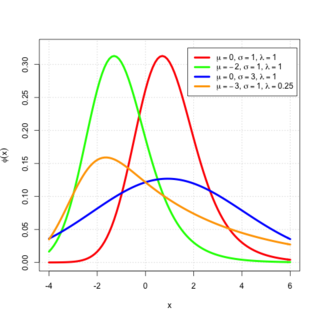
In probability theory, an exponentially modified Gaussian distribution describes the sum of independent normal and exponential random variables. An exGaussian random variable Z may be expressed as Z = X + Y, where X and Y are independent, X is Gaussian with mean μ and variance σ2, and Y is exponential of rate λ. It has a characteristic positive skew from the exponential component.
In applied mathematics and mathematical analysis, the fractal derivative or Hausdorff derivative is a non-Newtonian generalization of the derivative dealing with the measurement of fractals, defined in fractal geometry. Fractal derivatives were created for the study of anomalous diffusion, by which traditional approaches fail to factor in the fractal nature of the media. A fractal measure t is scaled according to tα. Such a derivative is local, in contrast to the similarly applied fractional derivative. Fractal calculus is formulated as a generalized of standard calculus
The Curie–von Schweidler law refers to the response of dielectric material to the step input of a direct current (DC) voltage first observed by Jacques Curie and Egon Ritter von Schweidler.
In physical oceanography and fluid mechanics, the Miles-Phillips mechanism describes the generation of wind waves from a flat sea surface by two distinct mechanisms. Wind blowing over the surface generates tiny wavelets. These wavelets develop over time and become ocean surface waves by absorbing the energy transferred from the wind. The Miles-Phillips mechanism is a physical interpretation of these wind-generated surface waves.
Both mechanisms are applied to gravity-capillary waves and have in common that waves are generated by a resonance phenomenon. The Miles mechanism is based on the hypothesis that waves arise as an instability of the sea-atmosphere system. The Phillips mechanism assumes that turbulent eddies in the atmospheric boundary layer induce pressure fluctuations at the sea surface. The Phillips mechanism is generally assumed to be important in the first stages of wave growth, whereas the Miles mechanism is important in later stages where the wave growth becomes exponential in time.
The Cole-Davidson equation is a model used to describe dielectric relaxation in glass-forming liquids. The equation for the complex permittivity is