Distance matrix

In mathematics, computer science and especially graph theory, a distance matrix is a square matrix (two-dimensional array) containing the distances, taken pairwise, between the elements of a set. ^[1] Depending upon the application involved, the distance being used to define this matrix may or may not be a metric. If there are N elements, this matrix will have size N×N. In graph-theoretic applications, the elements are more often referred to as points, nodes or vertices.

Non-metric distance matrix

In general, a distance matrix is a weighted adjacency matrix of some graph. In a network, a directed graph with weights assigned to the arcs, the distance between two nodes of the network can be defined as the minimum of the sums of the weights on the shortest paths joining the two nodes. ^[2] This distance function, while well defined, is not a metric. There need be no restrictions on the weights other than the need to be able to combine and compare them, so negative weights are used in some applications. Since paths are directed, symmetry can not be guaranteed, and if cycles exist the distance matrix may not be hollow.

An algebraic formulation of the above can be obtained by using the min-plus algebra. Matrix multiplication in this system is defined as follows: Given two n × n matrices A = (a_ij) and B = (b_ij), their distance product C = (c_ij) = A ⭑ B is defined as an n × n matrix such that

${\displaystyle c_{ij}=\min _{k=1}^{n}\{a_{ik}+b_{kj}\}.}$

Note that the off-diagonal elements that are not connected directly will need to be set to infinity or a suitable large value for the min-plus operations to work correctly. A zero in these locations will be incorrectly interpreted as an edge with no distance, cost, etc.

If W is an n × n matrix containing the edge weights of a graph, then W^k (using this distance product) gives the distances between vertices using paths of length at most k edges, and Wⁿ is the distance matrix of the graph.

An arbitrary graph G on n vertices can be modeled as a weighted complete graph on n vertices by assigning a weight of one to each edge of the complete graph that corresponds to an edge of G and zero to all other edges. W for this complete graph is the adjacency matrix of G. The distance matrix of G can be computed from W as above, however, Wⁿ calculated by the usual matrix multiplication only encodes the number of paths between any two vertices of length exactly n.

Metric distance matrix

The value of a distance matrix formalism in many applications is in how the distance matrix can manifestly encode the metric axioms and in how it lends itself to the use of linear algebra techniques. That is, if M = (x_ij) with 1 ≤ i, j ≤ N is a distance matrix for a metric distance, then

1. the entries on the main diagonal are all zero (that is, the matrix is a hollow matrix), i.e. x_ii = 0 for all 1 ≤ i ≤ N,
2. all the off-diagonal entries are positive (x_ij > 0 if i ≠ j), (that is, a non-negative matrix),
3. the matrix is a symmetric matrix (x_ij = x_ji), and
4. for any i and j, x_ij ≤ x_ik + x_kj for all k (the triangle inequality). This can be stated in terms of tropical matrix multiplication

When a distance matrix satisfies the first three axioms (making it a semi-metric) it is sometimes referred to as a pre-distance matrix. A pre-distance matrix that can be embedded in a Euclidean space is called a Euclidean distance matrix.

Another common example of a metric distance matrix arises in coding theory when in a block code the elements are strings of fixed length over an alphabet and the distance between them is given by the Hamming distance metric. The smallest non-zero entry in the distance matrix measures the error correcting and error detecting capability of the code.

Additive distance matrix

An additive distance matrix is a special type of matrix used in bioinformatics to build a phylogenetic tree. Let x be the lowest common ancestor between two species i and j, we expect M_ij = M_ix + M_xj. This is where the additive metric comes from. A distance matrix M for a set of species S is said to be additive if and only if there exists a phylogeny T for S such that:

• Every edge (u,v) in T is associated with a positive weight d_uv
• For every i,j ∈ S, M_ij equals the sum of the weights along the path from i to j in T

For this case, M is called an additive matrix and T is called an additive tree. Below we can see an example of an additive distance matrix and its corresponding tree:

Additive distance matrix (left) and its phylogeny tree (right)

Ultrametric distance matrix

The ultrametric distance matrix is defined as an additive matrix which models the constant molecular clock. It is used to build a phylogenetic tree. A matrix M is said to be ultrametric if there exists a tree T such that:

• M_ij equals the sum of the edge weights along the path from i to j in T
• A root of the tree can be identified with the distance to all the leaves being the same

Here is an example of an ultrametric distance matrix with its corresponding tree:

Bioinformatics

The distance matrix is widely used in the bioinformatics field, and it is present in several methods, algorithms and programs. Distance matrices are used to represent protein structures in a coordinate-independent manner, as well as the pairwise distances between two sequences in sequence space. They are used in structural and sequential alignment, and for the determination of protein structures from NMR or X-ray crystallography.

Sometimes it is more convenient to express data as a similarity matrix.

It is also used to define the distance correlation.

Sequence alignment

An alignment of two sequences is formed by inserting spaces in arbitrary locations along the sequences so that they end up with the same length and there are no two spaces at the same position of the two augmented sequences. ^[3] One of the primary methods for sequence alignment is dynamic programming. The method is used to fill the distance matrix and then obtain the alignment. In typical usage, for sequence alignment a matrix is used to assign scores to amino-acid matches or mismatches, and a gap penalty for matching an amino-acid in one sequence with a gap in the other.

Global alignment

The Needleman-Wunsch algorithm used to calculate global alignment uses dynamic programming to obtain the distance matrix.

Local alignment

The Smith-Waterman algorithm is also dynamic programming based which consists also in obtaining the distance matrix and then obtain the local alignment.

Multiple sequence alignment

Multiple sequence alignment is an extension of pairwise alignment to align several sequences at a time. Different MSA methods are based on the same idea of the distance matrix as global and local alignments.

• Center star method. This method defines a center sequence S_c which minimizes the distance between the sequence S_c and any other sequence S_i. Then it generates a multiple alignment M for the set of sequences S so that for every S_i the alignment distance d_M(S_c,S_i) is the optimal pairwise alignment. This method has the characteristic that the computed alignment for S whose sum-of-pair distance is at most twice the optimal multiple alignment.
• Progressive alignment method. This heuristic method to create MSA first aligns the two most related sequences, and then it progressively aligns the next two most related sequences until all sequences are aligned.

There are other methods that have their own program due to their popularity:

• ClustalW
• MUSCLE
• MAFFT
• MANGO
• And many more

MAFFT

Multiple alignment using fast Fourier transform (MAFFT) is a program with an algorithm based on progressive alignment, and it offers various multiple alignment strategies. First, MAFFT constructs a distance matrix based on the number of shared 6-tuples. Second, it builds the guide tree based on the previous matrix. Third, it clusters the sequences with the help of the fast Fourier transform and starts the alignment. Based on the new alignment, it reconstructs the guide tree and align again.

Phylogenetic analysis

Main article: Distance matrices in phylogeny

To perform phylogenetic analysis, the first step is to reconstruct the phylogenetic tree: given a collection of species, the problem is to reconstruct or infer the ancestral relationships among the species, i.e., the phylogenetic tree among the species. Distance matrix methods perform this activity.

Distance matrix methods

Distance matrix methods of phylogenetic analysis explicitly rely on a measure of "genetic distance" between the sequences being classified, and therefore require multiple sequences as an input. Distance methods attempt to construct an all-to-all matrix from the sequence query set describing the distance between each sequence pair. From this is constructed a phylogenetic tree that places closely related sequences under the same interior node and whose branch lengths closely reproduce the observed distances between sequences. Distance-matrix methods may produce either rooted or unrooted trees, depending on the algorithm used to calculate them. ^[4] Given n species, the input is an n × n distance matrix M where M_ij is the mutation distance between species i and j . The aim is to output a tree of degree 3 which is consistent with the distance matrix.

They are frequently used as the basis for progressive and iterative types of multiple sequence alignment. The main disadvantage of distance-matrix methods is their inability to efficiently use information about local high-variation regions that appear across multiple subtrees. ^[4] Despite potential problems, distance methods are extremely fast, and they often produce a reasonable estimate of phylogeny. They also have certain benefits over the methods that use characters directly. Notably, distance methods allow use of data that may not be easily converted to character data, such as DNA-DNA hybridization assays.

The following are distance based methods for phylogeny reconstruction:

• Additive tree reconstruction
• UPGMA
• Neighbor joining
• Fitch-Margoliash

Additive tree reconstruction

Additive tree reconstruction is based on additive and ultrametric distance matrices. These matrices have a special characteristic:

Consider an additive matrix M. For any three species i, j, k, the corresponding tree is unique. ^[3] Every ultrametric distance matrix is an additive matrix. We can observe this property for the tree below, which consists on the species i, j, k.

Phylogenetic tree from 3 species

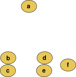
The additive tree reconstruction technique starts with this tree. And then adds one more species each time, based on the distance matrix combined with the property mentioned above. For example, consider an additive matrix M and 5 species a, b, c, d and e. First we form an additive tree for two species a and b. Then we chose a third one, let's say c and attach it to a point x on the edge between a and b. The edge weights are computed with the property above. Next we add the fourth species d to any of the edges. If we apply the property then we identify that d should be attached to only one specific edge. Finally, we add e following the same procedure as before.

UPGMA

The basic principle of UPGMA (Unweighted Pair Group Method with Arithmetic Mean) is that similar species should be closer in the phylogenetic tree. Hence, it builds the tree by clustering similar sequences iteratively. The method works by building the phylogenetic tree bottom up from its leaves. Initially, we have n leaves (or n singleton trees), each representing a species in S. Those n leaves are referred as n clusters. Then, we perform n-1 iterations. In each iteration, we identify two clusters C₁ and C₂ with the smallest average distance and merge them to form a bigger cluster C. If we suppose M is ultrametric, for any cluster C created by the UPGMA algorithm, C is a valid ultrametric tree.

Neighbor joining

Neighbor is a bottom-up clustering method. It takes a distance matrix specifying the distance between each pair of sequences. The algorithm starts with a completely unresolved tree, whose topology corresponds to that of a star network, and iterates over the following steps until the tree is completely resolved and all branch lengths are known:

1. Based on the current distance matrix calculate the matrix (defined below).
2. Find the pair of distinct taxa i and j (i.e. with) for which has its lowest value. These taxa are joined to a newly created node, which is connected to the central node.
3. Calculate the distance from each of the taxa in the pair to this new node.
4. Calculate the distance from each of the taxa outside of this pair to the new node.
5. Start the algorithm again, replacing the pair of joined neighbors with the new node and using the distances calculated in the previous step. ^[5]

Fitch-Margoliash

The Fitch–Margoliash method uses a weighted least squares method for clustering based on genetic distance. Closely related sequences are given more weight in the tree construction process to correct for the increased inaccuracy in measuring distances between distantly related sequences. The least-squares criterion applied to these distances is more accurate but less efficient than the neighbor-joining methods. An additional improvement that corrects for correlations between distances that arise from many closely related sequences in the data set can also be applied at increased computational cost. ^[6]

Data Mining and Machine Learning

Data Mining

A common function in data mining is applying cluster analysis on a given set of data to group data based on how similar or more similar they are when compared to other groups. Distance matrices became heavily dependent and utilized in cluster analysis since similarity can be measured with a distance metric. Thus, distance matrix became the representation of the similarity measure between all the different pairs of data in the set.

Hierarchical clustering

A distance matrix is necessary for traditional hierarchical clustering algorithms which are often heuristic methods employed in biological sciences such as phylogeny reconstruction. When implementing any of the hierarchical clustering algorithms in data mining, the distance matrix will contain all pair-wise distances between every point and then will begin to create clusters between two different points or clusters based entirely on distances from the distance matrix.

If N be the number of points, the complexity of hierarchical clustering is:

• Time complexity is ${\displaystyle O(N^{3})}$ due to the repetitive calculations done after every cluster to update the distance matrix
• Space complexity is ${\displaystyle O(N^{2})}$

Machine Learning

Distance metrics are a key part of several machine learning algorithms, which are used in both supervised and unsupervised learning. They are generally used to calculate the similarity between data points: this is where the distance matrix is an essential element. The use of an effective distance matrix improves the performance of the machine learning model, whether it is for classification tasks or for clustering. ^[7]

K-Nearest Neighbors

A distance matrix is utilized in the k-NN algorithm which is one of the slowest but simplest and most used instance-based machine learning algorithms that can be used both in classification and regression tasks. It is one of the slowest machine learning algorithms since each test sample's predicted result requires a fully computed distance matrix between the test sample and each training sample in the training set. Once the distance matrix is computed, the algorithm selects the K number of training samples that are the closest to the test sample to predict the test sample's result based on the selected set's majority (classification) or average (regression) value.

• Prediction time complexity is ${\displaystyle O(k*n*d)}$, to compute the distance between each test sample with every training sample to construct the distance matrix where:

1. k = number of nearest neighbors selected
2. n = size of the training set
3. d = number of dimensions being used for the data

This classification focused model predicts the label of the target based on the distance matrix between the target and each of the training samples to determine the K-number of samples that are the closest/nearest to the target.

Computer Vision

A distance matrix can be used in neural networks for 2D to 3D regression in image predicting machine learning models.

Information retrieval

Distance matrices using Gaussian mixture distance

• * Gaussian mixture distance for performing accurate nearest neighbor search for information retrieval. Under an established Gaussian finite mixture model for the distribution of the data in the database, the Gaussian mixture distance is formulated based on minimizing the Kullback-Leibler divergence between the distribution of the retrieval data and the data in database. In the comparison of performance of the Gaussian mixture distance with the well-known Euclidean and Mahalanobis distances based on a precision performance measurement, experimental results demonstrate that the Gaussian mixture distance function is superior in the others for different types of testing data.

Potential basic algorithms worth noting on the topic of information retrieval is Fish School Search algorithm an information retrieval that partakes in the act of using distance matrices in order for gathering collective behavior of fish schools. By using a feeding operator to update their weights

Eq. A:

${\displaystyle x_{i}(t+1)=x_{i}(t)-step_{vol}rand(0,1){\frac {x_{i}(t)-B(t)}{distance(x_{i}(t),B(t))}},}$

Eq. B:

${\displaystyle x_{i}(t+1)=x_{i}(t)+step_{vol}rand(0,1){\frac {x_{i}(t)-B(t)}{distance(x_{i}(t),B(t))}},}$

Stepvol defines the size of the maximum volume displacement preformed with the distance matrix, specifically using a Euclidean distance matrix.

Evaluation of the similarity or dissimilarity of Cosine similarity and Distance matrices

Conversion formula between cosine similarity and Euclidean Distance

• * While the Cosine similarity measure is perhaps the most frequently applied proximity measure in information retrieval by measuring the angles between documents in the search space on the base of the cosine. Euclidean distance is invariant to mean-correction. The sampling distribution of a mean is generated by repeated sampling from the same population and recording of the sample means obtained. This forms a distribution of different means, and this distribution has its own mean and variance. For the data which can be negative as well as positive, the null distribution for cosine similarity is the distribution of the dot product of two independent random unit vectors. This distribution has a mean of zero and a variance of 1/n. While Euclidean distance will be invariant to this correction.

Clustering Documents

The implementation of hierarchical clustering with distance-based metrics to organize and group similar documents together will require the need and utilization of a distance matrix. The distance matrix will represent the degree of association that a document has with another document that will be used to create clusters of closely associated documents that will be utilized in retrieval methods of relevant documents for a user's query.

Isomap

Isomap incorporates distance matrices to utilize geodesic distances to able to compute lower-dimensional embeddings. This helps to address a collection of documents that reside within a massive number of dimensions and empowers to perform document clustering.

Neighborhood Retrieval Visualizer (NeRV)

An algorithm used for both unsupervised and supervised visualization that uses distance matrices to find similar data based on the similarities shown on a display/screen.

The distance matrix needed for Unsupervised NeRV can be computed through fixed input pairwise distances.

The distance matrix needed for Supervised NeRV requires formulating a supervised distance metric to be able to compute the distance of the input in a supervised manner.

Chemistry

The distance matrix is a mathematical object widely used in both graphical-theoretical (topological) and geometric (topographic) versions of chemistry. ^[8] The distance matrix is used in chemistry in both explicit and implicit forms.

Interconversion mechanisms between two permutational isomers

Distance matrices were used as the main approach to depict and reveal the shortest path sequence needed to determine the rearrangement between the two permutational isomers.

Distance Polynomials and Distance Spectra

Explicit use of Distance matrices is required in order to construct the distance polynomials and distance spectra of molecular structures.

Structure-property model

Implicit use of Distance matrices was applied through the use of the distance based metric Weiner number/Weiner Index which was formulated to represent the distances in all chemical structures. The Weiner number is equal to half-sum of the elements of the distance matrix.

Conversion formula between Weiner Number and Distance Matrix

Graph-theoretical Distance matrix

Distance matrix in chemistry that are used for the 2-D realization of molecular graphs, which are used to illustrate the main foundational features of a molecule in a myriad of applications.

Labeled tree representation of C₆H₁₄'s carbon skeleton based on its distance matrix

1. Creating a label tree that represents the carbon skeleton of a molecule based on its distance matrix. The distance matrix is imperative in this application because similar molecules can have a myriad of label tree variants of their carbon skeleton. The labeled tree structure of hexane (C₆H₁₄) carbon skeleton that is created based on the distance matrix in the example, has different carbon skeleton variants that affect both the distance matrix and the labeled tree
2. Creating a labeled graph with edge weights, used in chemical graph theory, that represent molecules with hetero-atoms.
3. Le Verrier-Fadeev-Frame (LVFF) method is a computer oriented used to speed up the process of detecting the graph center in polycyclic graphs. However, LVFF requires the input to be a diagonalized distance matrix which is easily resolved by implementing the Householder tridiagonal-QL algorithm that takes in a distance matrix and returns the diagonalized distance needed for the LVFF method.

Geometric-Distance Matrix

Geometric distance matrix for 2,4-dimethylhexane

While the graph-theoretical distance matrix 2-D captures the constitutional features of the molecule, its three-dimensional (3D) character is encoded in the geometric-distance matrix. The geometric-distance matrix is a different type of distance matrix that is based on the graph-theoretical distance matrix of a molecule to represent and graph the 3-D molecule structure. ^[8] The geometric-distance matrix of a molecular structure G is a real symmetric n x n matrix defined in the same way as a 2-D matrix. However, the matrix elements D_ij will hold a collection of shortest Cartesian distances between i and j in G. Also known as topographic matrix, the geometric-distance matrix can be constructed from the known geometry of the molecule. As an example, the geometric-distance matrix of the carbon skeleton of 2,4-dimethylhexane is shown below:

Other Applications

Time Series Analysis

Dynamic Time Warping distance matrices are utilized with the clustering and classification algorithms of a collection/group of time series objects.

Examples

For example, suppose these data are to be analyzed, where pixel Euclidean distance is the distance metric.

Raw data

The distance matrix would be:

	a	b	c	d	e	f
a	0	184	222	177	216	231
b	184	0	45	123	128	200
c	222	45	0	129	121	203
d	177	123	129	0	46	83
e	216	128	121	46	0	83
f	231	200	203	83	83	0

These data can then be viewed in graphic form as a heat map. In this image, black denotes a distance of 0 and white is maximal distance.

Graphical View

See also

• Computer Vision
• Data clustering
• Distance set
• Hollow matrix
• Min-plus matrix multiplication

References

1. Weyenberg, G., & Yoshida, R. (2015). Reconstructing the phylogeny: Computational methods. In Algebraic and Discrete Mathematical methods for modern Biology (pp. 293–319). Academic Press.
2. Frank Harary, Robert Z. Norman and Dorwin Cartwright (1965) Structural Models: An Introduction to the Theory of Directed Graphs, pages 134–8, John Wiley & Sons MR 0184874
3. Sung, Wing-Kin (2010). Algorithms in bioinformatics: A practical introduction. Chapman & Hall. p. 29. ISBN   978-1-4200-7033-0.
4. Felsenstein, Joseph (2003). Inferring phylogenies. Sinauer Associates. ISBN   9780878931774.
5. Saitou, Naruya (1987). "The neighbor-joining method: A new method for reconstructing phylogenetic trees". Molecular Biology and Evolution. 4 (4): 406–425. doi: 10.1093/oxfordjournals.molbev.a040454 . PMID   3447015.
6. Fitch, Walter M. (1967). "Construction of Phylogenetic Trees: A method based on mutation distances as estimated from cytochrome c sequences is of general applicability". Science. 155 (3760): 279–284. doi:10.1126/science.155.3760.279. PMID   5334057.
7. "4 types of distance metrics in machine learning". February 25, 2020.
8. Mihalic, Zlatko (1992). "The distance matrix in chemistry". Journal of Mathematical Chemistry. 11: 223–258. doi:10.1007/BF01164206. S2CID   121181446.