Numerical modeling (geology)

Last updated
Simulation of seismic wave propagation in global scale using supercomputer to solve wave equations Global Seismic Wave Propagation Simulation.gif
Simulation of seismic wave propagation in global scale using supercomputer to solve wave equations

In geology, numerical modeling is a widely applied technique to tackle complex geological problems by computational simulation of geological scenarios.

Contents

Numerical modeling uses mathematical models to describe the physical conditions of geological scenarios using numbers and equations. [2] Nevertheless, some of their equations are difficult to solve directly, such as partial differential equations. With numerical models, geologists can use methods, such as finite difference methods, to approximate the solutions of these equations. Numerical experiments can then be performed in these models, yielding the results that can be interpreted in the context of geological process. [2] Both qualitative and quantitative understanding of a variety of geological processes can be developed via these experiments. [3]

Numerical modelling has been used to assist in the study of rock mechanics, thermal history of rocks, movements of tectonic plates and the Earth's mantle. Flow of fluids is simulated using numerical methods, and this shows how groundwater moves, or how motions of the molten outer core yields the geomagnetic field.

History

Prior to the development of numerical modeling, analog modeling, which simulates nature with reduced scales in mass, length, and time, was one of the major ways to tackle geological problems, [4] [5] for instance, to model the formation of thrust belts. [6] Simple analytic or semi-analytic mathematical models were also used to deal with relatively simple geological problems quantitatively. [2]

In the late 1960s to 1970s, following the development of finite-element methods in solving continuum mechanics problems for civil engineering, numerical methods were adapted for modeling complex geological phenomena, [5] [7] for example, folding [8] [9] and mantle convection. [10] With advances in computer technology, the accuracy of numerical models has been improved. [2] Numerical modeling has become an important tool for tackling geological problems, [2] especially for the parts of the Earth that are difficult to observe directly, such as the mantle and core. Yet analog modeling is still useful in modeling geological scenarios that are difficult to capture in numerical models, and the combination of analog and numerical modeling can be useful to improve understanding of the Earth's processes. [11]

Components

Steps in numerical modeling. The first step in numerical modeling is to capture the actual geological scenario quantitatively. For example, in mantle convection modeling, heat equations are used to describe the heat energy circulating in the system while Navier-Stokes equations describe the flow of viscous fluid (the mantle rock). Second, since these equations are difficult to solve, discretization and numerical methods are chosen to make an approximation to the governing equations. Then, algorithms in the computer can calculate the approximated solutions. Finally, interpretation can be made from those solutions. For instance, in mantle convection modeling, the flow of mantle can first be visualized. Then, the relationship between the patterns of flow and the input parameters may be concluded. Flowchart of Numerical modelling.svg
Steps in numerical modeling. The first step in numerical modeling is to capture the actual geological scenario quantitatively. For example, in mantle convection modeling, heat equations are used to describe the heat energy circulating in the system while Navier–Stokes equations describe the flow of viscous fluid (the mantle rock). Second, since these equations are difficult to solve, discretization and numerical methods are chosen to make an approximation to the governing equations. Then, algorithms in the computer can calculate the approximated solutions. Finally, interpretation can be made from those solutions. For instance, in mantle convection modeling, the flow of mantle can first be visualized. Then, the relationship between the patterns of flow and the input parameters may be concluded.

A general numerical model study usually consists of the following components: [12] [2]

  1. Mathematical model is a simplified description of the geological problem, such as equations and boundary conditions. [2] These governing equations of the model are often partial differential equations that are difficult to solve directly since it involves the derivative of the function, [13] for example, the wave equation. [2]
  2. Discretization methods and numerical methods convert those governing equations in the mathematical models to discrete equations. [2] These discrete equations can approximate the solution of the governing equations. [2] Common methods include the finite element, finite difference, or finite volume method that subdivide the object of interest into smaller pieces (element) by mesh. These discrete equations can then be solved in each element numerically. [2] The discrete element method uses another approach, this method reassembling the object of interest from numerous tiny particles. Simple governing equations are then applied to the interactions between particles.
  3. Algorithms are computer programs that compute the solution using the idea of the above numerical methods. [2]
  4. Interpretations are made from the solutions given by the numerical models. [2]

Properties

A good numerical model usually has some of the following properties: [12] [2]

Computation

The following are some key aspects of ideas in developing numerical models in geology. First, the way to describe the object and motion should be decided (kinematic description). Then, governing equations that describe the geological problems are written, for example, the heat equations describe the flow of heat in a system. Since some of these equations cannot be solved directly, numerical methods are used to approximate the solution of the governing equations.

Kinematic descriptions

In numerical models and mathematical models, there are two different approaches to describe the motion of matter: Eulerian and Lagrangian. [14] In geology, both approaches are commonly used to model fluid flow like mantle convection, where an Eulerian grid is used for computation and Lagrangian markers are used to visualize the motion. [2] Recently, there have been models that try to describe different parts using different approaches to combine the advantages of these two approaches. This combined approach is called the arbitrary Lagrangian-Eulerian approach. [15]

Eulerian

The Eulerian approach considers the changes of the physical quantities, such as mass and velocity, of a fixed location with time. [14] It is similar to looking at how river water flows past a bridge. Mathematically, the physical quantities can be expressed as a function of location and time. This approach is useful for fluid and homogeneous (uniform) materials that have no natural boundary. [16]

Lagrangian

The Lagrangian approach, on the other hand, considers the change of physical quantities, such as the volume, of fixed elements of matter over time. [14] It is similar to looking at a certain collection of water molecules as they flow downstream in a river. Using the Lagrangian approach, it is easier to follow solid objects which have natural boundary to separate them from the surrounding. [16]

Governing equations

Following are some basic equations that are commonly used to describe physical phenomena, for example, how the matter in a geologic system moves or flows and how heat energy is distributed in a system. These equations are usually the core of the mathematical model.

Continuity equation

The continuity equation is a mathematical version of stating that the geologic object or medium is continuous, which means no empty space can be found in the object. [17] This equation is commonly used in numerical modeling in geology. [17]

One example is the continuity equation of mass of fluid. Based on the law of conservation of mass, for a fluid with density at position in a fixed volume of fluid, the rate of change of mass is equal to the outward fluid flow across the boundary :

where is the volume element and is the velocity at .

In Lagrangian form: [2]

In Eulerian form: [2]

This equation is useful when the model involves continuous fluid flow, like the mantle is over geological time scales. [2]

Momentum equation

The momentum equation describes how matter moves in response to force applied. It is an expression of Newton's second law of motion. [17]

Consider a fixed volume of matter. By the law of conservation of momentum, the rate of change of volume is equal to: [2]

  • external force applied on the element
  • plus normal stress and shear stress applied on the surface bounding the element
  • minus the momentum moving out of the element on that surface

where is the volume element, is the velocity.

After simplifications and integrations, for any volume , the Eulerian form of this equation is: [2] [17]

Heat equation

The heat equations describe how heat energy flows in a system.

From the law of conservation of energy, the rate of change of energy of a fixed volume of mass is equal to: [2]

  • work done at the boundary
  • plus work done by external force in the volume
  • minus heat conduction across boundary
  • minus heat convection across boundary
  • plus heat produced internally

Mathematically:

where is the volume element, is the velocity, is the temperature, is the conduction coefficient and is the rate of heat production. [2]

Numerical methods

An example of 2D finite element mesh. The domain is subdivided into numerous non-overlapping triangles (elements). Nodes are the vertices of the triangles. Example of 2D mesh.png
An example of 2D finite element mesh. The domain is subdivided into numerous non-overlapping triangles (elements). Nodes are the vertices of the triangles.

Numerical methods are techniques to approximate the governing equations in the mathematical models.

Common numerical methods include finite element method, spectral method, finite difference method, and finite volume method. These methods are used to approximate the solution of governing differential equations in the mathematical model by dissecting the domain into meshes or grids and applying simpler equations to individual elements or nodes in the mesh. [2] [18]

Approximating wave equations using the finite element method. The domain is subdivided into numerous triangles. The values of the nodes in the mesh are calculated, showing how a wave propagates in the region.

The discrete element method uses another approach. The object is considered an assemblage of small particles. [19]

Finite element method

The finite element method subdivides the object (or domain) into smaller, non-overlapping elements (or subdomains) and these elements are connected at the nodes. The solution for the partial differential equations are then approximated by simpler element equations, usually polynomials. [2] [20] [21] Then these element equations are combined into equations for the entire object, i.e. the contribution of each element is summed up to model the response of the whole object. [2] [20] [21] This method is commonly used to solve mechanical problems. [21] The following are the general steps of using the finite element method: [21]

  1. Select the element type and subdivide the object. Common element types include triangular, quadrilateral, tetrahedral, etc. [21] Different types of elements should be chosen for different problems.
  2. Decide the function of displacement. The function of displacement governs how the elements move. Linear, quadratic, or cubic polynomial functions are commonly used. [21]
  3. Decide the displacement-strain relation. The displacement of the element changes or deforms the element's shape in what is technically called strain. This relation calculates how much strain the element experienced due to the displacement. [21]
  4. Decide the strain-stress relation. The deformation of the element induces stress to the element, which is the force applied to the element. This relation calculates the amount of stress experienced by the element due to the strain. One of the examples of this relation is Hooke's law. [21]
  5. Derive equations of stiffness and stiffness matrix for elements. The stress also causes the element to deform; the stiffness (the rigidity) of the elements indicates how much it will deform in response to the stress. The stiffness of the elements in different directions is represented in matrix form for simpler operation during calculation. [21]
  6. Combine the element equations into global equations. The contributions of every element are summed up to a set of equations that describe the whole system. [21]
  7. Apply boundary conditions. The predefined conditions at the boundary, such as temperature, stress, and other physical quantities are introduced to the boundary of the system. [21]
  8. Solve for displacement. As time evolves, the displacement of the elements are solved step by step. [21]
  9. Solve for strains and stress. After the displacement is calculated, the strains and stress are computed using the relations in steps 3 and 4. [21]
Solution of Burgers Equation, which describes how shock waves behave, using spectral method. The domain is first subdivided into rectangular mesh. The idea of this method is similar to the finite element method. Inviscid Burgers Equation in Two Dimensions.gif
Solution of Burgers Equation, which describes how shock waves behave, using spectral method. The domain is first subdivided into rectangular mesh. The idea of this method is similar to the finite element method.

Spectral method

The spectral method is similar to the finite element method. [22] [23] The major difference is that spectral method uses basis functions, possibly by using a Fast Fourier Transformation (FFT) that approximates the function by the sum of numerous simple functions. [22] [23] These kinds of basis functions can then be applied to the whole domain and approximate the governing partial differential equations. [2] [22] [23] Therefore, each calculation takes the information from the whole domain into account while the finite element method only takes the information from the neighborhood. [22] [23] As a result, the spectral method converges exponentially and is suitable for solving problems involving a high variability in time or space. [22] [23]

Finite volume method

The finite volume method is also similar to the finite element method. It also subdivides the object of interest into smaller volumes (or elements), then the physical quantities are solved over the control volume as fluxes of these quantities across the different faces. [2] [24] The equations used are usually based on the conservation or balance of physical quantities, like mass and energy. [24] [25]

The finite volume method can be applied on irregular meshes like the finite element method. The element equations are still physically meaningful. However, it is difficult to get better accuracy, as the higher order version of element equations are not well-defined. [2] [24] [25]

Finite difference method

The finite difference method approximates differential equations by approximating the derivative with a difference equation, which is the major method to solve partial differential equations. [26] [27] [28] [29]

Finite difference method Finite difference method 2.svg
Finite difference method

Consider a function with single-valued derivatives that are continuous and finite functions of , according to Taylor's theorem: [30]

and

Summing up the above expressions: [30]

Ignore the terms with higher than 4th power of , then: [30]

The above is the central-difference approximation of the derivatives, [30] which can also be approximated by forward-difference:

or backward-difference:

The accuracy of the finite differences can be improved when more higher order terms are used.

Discrete element method

An example of model using discrete element method, which uses photo of Peter A. Cundall to initiate the particles Cundall DEM.gif
An example of model using discrete element method, which uses photo of Peter A. Cundall to initiate the particles

The discrete element method, sometimes called distinct element method, is usually used to model discontinuous materials, such as rocks with fractures like joints and bedding, since it can explicitly model the properties of discontinuities. [19] This method was developed to simulate rock mechanics problems at the beginning. [19] [31]

The main idea of this method is to model the objects as an assemblage of smaller particles, [19] which is similar to building a castle out of sand. These particles are of simple geometry, such as a sphere. The physical quantities of each particle, such as velocity, are continuously updated at the contacts between them. [19] This model is relatively computationally intensive, as a large quantity of particles needs to be used, [19] especially for large-scale models, like a slope. [32] Therefore, this model is usually applied to small-scale objects.

Bonded-particle model

There are objects that are not composed of granular materials, such as crystalline rocks composed of mineral grains that stick to each other or interlock with each other. Some bonding between particles is added to model this cohesion or cementation between particles. This kind of model is also called a bonded-particle model. [33] [34] [35]

Applications

Numerical modeling can be used to model problems in different fields of geology at various scales, such as engineering geology, geophysics, geomechanics, geodynamics, rock mechanics, hydrogeology, and stratigraphy. [36] The following are some examples of applications of numerical modeling in geology.

Specimen to outcrop scale

Rock mechanics

Numerical modeling has been widely applied in different fields of rock mechanics. [3] Rock is a material that is difficult to model because rock are usually: [3]

  • Discontinuous: There are numerous fractures and micro-fractures in a rock mass [37] and the space in the rock mass maybe filled with other substances like air and water. [3] A complex model is needed to fully capture these discontinuities, since the discontinuities have great effects on the rock mass. [3]
  • Anisotropic: The properties of rock mass, such as permeability (the ability to allow fluid to flow through), may vary in different directions. [3] [37]
  • Inhomogeneous: The properties of different portions of the rock mass may be different. [3] [37] For example, the physical properties of quartz grains and feldspar grains are different in granite. [38] [39]
  • Not elastic: Rock cannot perfectly revert to its original shape after stress is removed. [37] [3]

In order to model the behaviors of rock, a complex model that takes all the above characteristics into account is needed. [3] There are many models modeling rock as a continuum using methods like finite difference, finite element, and boundary element methods. One of the disadvantages is that the ability of modeling cracks and other discontinuities is usually limited in these models. [40] Models that model rock as a discontinuum, using methods like discrete element and discrete fracture network methods, are also commonly employed. [3] [35] Combinations of both methods have also been developed. [3]

Numerical modeling enhances the understanding of mechanical processes in rock by conducting numerical experiments, and is useful for design and construction works. [3]

Regional-scale

Thermochronology

Numerical modeling has been used to predict and describe the thermal history of the Earth's crust, which allows geologists to improve their interpretation of thermochronological data. [41] Thermochronology can indicate the time at which a rock cooled below a particular temperature. [42] Geologic events, like the development of a faults and surface erosion, can change the thermochronological pattern of samples collected on the surface, and it is possible to constrain the geologic events by these data. [42] Numerical modeling can be used to predict the pattern.

The difficulties of thermal modeling of the Earth's crust mainly involve the irregularity and the changes of the Earth's surface (mainly erosion) through time. Therefore, in order to model the morphological changes of the Earth's surface, the models need to solve heat equations with boundary conditions that change with time and have irregular meshes. [43]

Pecube

Pecube is one of the numerical models developed to predict the thermochronological pattern. [43] It solves the following generalized heat transfer equation with advection using finite element method. [41] The first three terms on the right-hand side are the heat transferred by conduction in , and directions while is the advection.

After the temperature field is constructed in the model, particle paths are traced and the cooling history of the particles can be obtained. [41] The pattern of thermochronological age can then be computed. [41]

A cross-section showing the thermal and exhumation patterns of the crust generated by the movement of a fault. The simulation is generated by Pecube [Helsinki University Geodynamics Group (HUGG) version]. The model is three-dimensional; the figure shows a slice of the model for simplicity. In the figure, the white line indicates the fault. The small black arrows indicate the direction of movement of the material at that point. The red lines are isotherm (the point of the line are of same temperature). The Pecube model uses both Eulerian and Lagrangian approaches. The fault can be regarded as stationary and the crust is moving. Initially, the temperature of the crust depends on the depth. The deeper the depth, the hotter the material. During this event, the motion of crust along the fault moves the material with different temperatures. In the hanging wall (the block above the fault), hotter material from deeper depth moves towards the surface; while the cooler material at shallower depth in the footwall (the block below the fault) moves deeper. The flow of material changes the thermal pattern (the isotherm bends across the fault) of the crust, which may reset the thermochronometers in the rock. On the other hand, the exhumation rate also affects the thermochronometers in the rock. A positive rate of exhumation indicates the rock is moving towards the surface, while a negative rate of exhumation indicate the rock is moving downwards. The fault geometry impacts the pattern exhumation rate on the surface. Thermal and exhumation pattern due to a fault generated by Helsinki University Geodynamics Group (HUGG) version of the thermokinematic and thermochronometer age prediction program Pecube (Pecube-HUGG).gif
A cross-section showing the thermal and exhumation patterns of the crust generated by the movement of a fault. The simulation is generated by Pecube [Helsinki University Geodynamics Group (HUGG) version]. The model is three-dimensional; the figure shows a slice of the model for simplicity. In the figure, the white line indicates the fault. The small black arrows indicate the direction of movement of the material at that point. The red lines are isotherm (the point of the line are of same temperature). The Pecube model uses both Eulerian and Lagrangian approaches. The fault can be regarded as stationary and the crust is moving. Initially, the temperature of the crust depends on the depth. The deeper the depth, the hotter the material. During this event, the motion of crust along the fault moves the material with different temperatures. In the hanging wall (the block above the fault), hotter material from deeper depth moves towards the surface; while the cooler material at shallower depth in the footwall (the block below the fault) moves deeper. The flow of material changes the thermal pattern (the isotherm bends across the fault) of the crust, which may reset the thermochronometers in the rock. On the other hand, the exhumation rate also affects the thermochronometers in the rock. A positive rate of exhumation indicates the rock is moving towards the surface, while a negative rate of exhumation indicate the rock is moving downwards. The fault geometry impacts the pattern exhumation rate on the surface.

Hydrogeology

In hydrogeology, groundwater flow is often modeled numerically by the finite element method [46] [47] [48] and finite difference method. [49] These two methods have been shown to produce similar results if the mesh is fine enough. [50] [51]

Finite difference grid used in MODFLOW MODFLOW 3D grid.png
Finite difference grid used in MODFLOW
MODFLOW

One of the well-known programs in modeling groundwater flow is MODFLOW, developed by the United States Geological Survey. It is a free and open-source program that uses the finite difference method as the framework to model groundwater conditions. The recent development of related programs offers more features, including: [52] [53]

  • Interactions between groundwater and surface-water systems [52]
  • Transportation of solutes [52]
  • Flow of fluid with variable density, such as salt water [52]
  • Compaction of aquifer systems [52]
  • Subsidence of land [52]
  • Management of groundwater [52]

Crustal dynamics

The rheology (response of materials to stress) of crust and the lithosphere is complex, since a free surface (the land surface) and the plasticity and elasticity of the crustal materials need to be considered. [2] Most of the models use finite element methods with a Lagrangian mesh. [2] One usage is the study of deformation and kinematics of subduction. [54] [55]

FLAC

The Fast Lagrangian Analysis of Continua (FLAC) is one of the most popular approaches in modeling crustal dynamics. [2] The approach is fast as it solves the equations of momentum and continuity without using a matrix, hence it is fast but time steps must be small enough. [56] The approach has been used in 2D, [57] [58] [59] 2.5D, [60] and 3D [61] studies of crustal dynamics, in which the 2.5D results were generated by combining multiple slices of two-dimensional results. [2]

This figure shows the setup of the numerical model used in the study of tectonic evolution of the Cathaysia Block, which makes up the southeast part of the South China carton. This model uses the code called Flamar, which is a FLAC-like code that combines finite difference and finite element methods. The element used in this Lagrangian mesh is quadrilateral. The boundary conditions applied to the land surface are free, which is affected by erosion and sediment deposition. The boundary on the sides is at constant velocity, which will push the crust to subduct. The boundary condition used at the bottom is called "Winkler's pliable basement". It is at hydrostatic equilibrium and it allows the base to slip freely horizontally. Boundary conditions applied to models.tif
This figure shows the setup of the numerical model used in the study of tectonic evolution of the Cathaysia Block, which makes up the southeast part of the South China carton. This model uses the code called Flamar, which is a FLAC-like code that combines finite difference and finite element methods. The element used in this Lagrangian mesh is quadrilateral. The boundary conditions applied to the land surface are free, which is affected by erosion and sediment deposition. The boundary on the sides is at constant velocity, which will push the crust to subduct. The boundary condition used at the bottom is called "Winkler's pliable basement". It is at hydrostatic equilibrium and it allows the base to slip freely horizontally.

Global-scale

Mantle convection

A simulation of mantle convection in a form of a quarter of 2D annulus using ASPECT. In the model, the temperature of the core-mantle boundary (inner boundary) is a constant of 4273 K (about 4000degC), while that at the boundary between crust and mantle (outer boundary) is 973 K (about 700degC). The mesh in the simulation changes over time. The code uses adaptive mesh refinement, the mesh is finer in the areas that need more accurate calculation, such as the rising plumes, while the mesh is coarser in other area to save the computational power. In the figure, red color indicates a warmer temperature while blue color indicate a cooler temperature; hot material rises from the core mantle boundary due to lower density. When the hot material reaches the outer boundary, it starts to move in horizontally and eventually sinks due to cooling. Simulation of 2D mantle convection in a quarter of annulus using ASPECT mantle convection code.gif
A simulation of mantle convection in a form of a quarter of 2D annulus using ASPECT. In the model, the temperature of the core-mantle boundary (inner boundary) is a constant of 4273 K (about 4000°C), while that at the boundary between crust and mantle (outer boundary) is 973 K (about 700°C). The mesh in the simulation changes over time. The code uses adaptive mesh refinement, the mesh is finer in the areas that need more accurate calculation, such as the rising plumes, while the mesh is coarser in other area to save the computational power. In the figure, red color indicates a warmer temperature while blue color indicate a cooler temperature; hot material rises from the core mantle boundary due to lower density. When the hot material reaches the outer boundary, it starts to move in horizontally and eventually sinks due to cooling.

There are many attempts to model mantle convection.

Finite element, [65] finite volume, finite difference [66] and spectral methods have all been used in modeling mantle convection, and almost every model used an Eulerian grid. [2] Due to the simplicity and speed of the finite-difference and spectral methods, they were used in some early models, but finite-element or finite volume methods were generally adopted in the 2010s. [2] Many benchmark papers have investigated the validity of these numerical models. [2] [67] [68] [69] [70] [71] [72] Current approaches mostly uses a fixed and uniform grid. [2] Grid refinement, in which the size of the elements is reduced in the part that requires more accurate approximation, is possibly the direction of future development in numerical modeling of mantle convection. [2] [73]

Finite difference approach

In the 1960s to 1970s, mantle convection models using the finite difference approach usually used second-order finite differences. [2] [67] Stream functions were used to remove the effect of pressure and reduce the complexity of the algorithm. [2] Due to the advancement in computer technology, finite differences with higher order terms are now used to generate a more accurate result. [2] [74]

Finite volume approach

Mantle convection modeled by finite volume approach is often based on the balance between pressure and momentum. The equations derived are the same as the finite difference approach using a grid with staggered velocity and pressure, in which the values of velocity and the pressure of each element are located at different points. [2] This approach can maintain the coupling between velocity and pressure. [2]

Multiple codes are developed based on this finite difference/finite volume approach. [2] [75] [76] [77] [78] [66] [79] In modeling three-dimensional geometry of the Earth, since the parameters of mantles vary at different scales, multigrid, which means using different grid sizes for different variables, is applied to overcome the difficulties. [2] Examples include the cubed sphere grid, [80] [81] 'Yin-Yang' grid, [82] [83] [84] and spiral grid. [85]

Finite element approach

In the finite element approach, stream functions are also often used to reduce the complexity of the equations. [2] ConMan, [86] modeling two-dimensional incompressible flow in the mantle, was one of the popular codes for modeling mantle convection in the 1990s. [87] [2] Citcom, an Eulerian mutlgrid finite element model, is one of the most popular programs [2] to model mantle convection in 2D [88] and 3D. [89]

Spectral method

The spectral method in mantle convection breaks down the three-dimensional governing equation into several one-dimensional equations, which solves the equations much faster. It was one of the popular approaches in early models of mantle convection. [2] Many program were developed using this method during the 1980s to early 2000s. [2] [90] [91] [92] [93] [94] [95] [96] However, the lateral changes of viscosity of mantle are difficult to manage in this approach, and other methods became more popular in the 2010s. [2]

The Earth consists of several plates. Numerical models can be used to model the kinematics of plates. Tectonic plates.png
The Earth consists of several plates. Numerical models can be used to model the kinematics of plates.

Plate tectonics

Plate tectonics is a theory suggesting that the Earth's lithosphere is essentially composed of plates floating on the mantle. [97] The mantle convection model is fundamental in modeling the plates floating on it, and there are two major approaches to incorporate the plates into this model: rigid-block approach and rheological approach. [2] The rigid-block approach assumes the plates are rigid, which means the plates keep their shape and do not deform, just like some wooden blocks floating on water. In contrast, the rheological approach models the plates as a highly viscous fluid in which the equations applied to the lithosphere beneath also apply to the plates on top. [2]

Geodynamo

Numerical models have been made to verify the geodynamo theory, a theory that posits that the geomagnetic field is generated by the motion of conductive iron and nickel fluid in the Earth's core. [2] [98]

Modeling of the flow of Earth's liquid outer core is difficult because: [2]

Most of the models use the spectral method to simulate the geodynamo, [2] [99] for example the Glatzmaier-Roberts model. [100] [101] Finite difference method has also been used in the model by Kageyama and Sato. [99] [102] Some study also tried other methods, like finite volume [103] and finite element methods. [104]

A numerical geodynamo model (Glatzmaier-Roberts model) showing the magnetic field generated by the flowing liquid outer core. This figure shows how the magnetic field of the Earth behaves during a magnetic reversal. NASA 54559main comparison1 strip.gif
A numerical geodynamo model (Glatzmaier-Roberts model) showing the magnetic field generated by the flowing liquid outer core. This figure shows how the magnetic field of the Earth behaves during a magnetic reversal.

Seismology

Simulation of seismic wave propagation through the Earth. Global Seismic Wave Propagation Simulation.gif
Simulation of seismic wave propagation through the Earth.

Finite difference methods have been widely used in simulations of the propagation of seismic waves. [106] [107] [108] However, due to limitations in computation power, in some models, the spacing of the mesh is too large (compared with the wavelength of the seismic waves) so that the results are inaccurate due to grid dispersion, in which the seismic waves with different frequencies separate. [106] [109] Some researchers suggest using the spectral method to model seismic wave propagation. [106] [110]

Errors and limitations

Sources of error

While numerical modeling provides accurate quantitative estimation to geological problems, there is always a difference between the actual observation and the modeling results due to: [2]

Limitations

Apart from the errors, there are some limitations in using numerical models:

See also

Related Research Articles

In fluid mechanics, the Rayleigh number (Ra, after Lord Rayleigh) for a fluid is a dimensionless number associated with buoyancy-driven flow, also known as free (or natural) convection. It characterises the fluid's flow regime: a value in a certain lower range denotes laminar flow; a value in a higher range, turbulent flow. Below a certain critical value, there is no fluid motion and heat transfer is by conduction rather than convection. For most engineering purposes, the Rayleigh number is large, somewhere around 106 to 108.

<span class="mw-page-title-main">Dynamo theory</span> Mechanism by which a celestial body generates a magnetic field

In physics, the dynamo theory proposes a mechanism by which a celestial body such as Earth or a star generates a magnetic field. The dynamo theory describes the process through which a rotating, convecting, and electrically conducting fluid can maintain a magnetic field over astronomical time scales. A dynamo is thought to be the source of the Earth's magnetic field and the magnetic fields of Mercury and the Jovian planets.

The finite volume method (FVM) is a method for representing and evaluating partial differential equations in the form of algebraic equations. In the finite volume method, volume integrals in a partial differential equation that contain a divergence term are converted to surface integrals, using the divergence theorem. These terms are then evaluated as fluxes at the surfaces of each finite volume. Because the flux entering a given volume is identical to that leaving the adjacent volume, these methods are conservative. Another advantage of the finite volume method is that it is easily formulated to allow for unstructured meshes. The method is used in many computational fluid dynamics packages. "Finite volume" refers to the small volume surrounding each node point on a mesh.

<span class="mw-page-title-main">Boltzmann equation</span> Equation of statistical mechanics

The Boltzmann equation or Boltzmann transport equation (BTE) describes the statistical behaviour of a thermodynamic system not in a state of equilibrium; it was devised by Ludwig Boltzmann in 1872. The classic example of such a system is a fluid with temperature gradients in space causing heat to flow from hotter regions to colder ones, by the random but biased transport of the particles making up that fluid. In the modern literature the term Boltzmann equation is often used in a more general sense, referring to any kinetic equation that describes the change of a macroscopic quantity in a thermodynamic system, such as energy, charge or particle number.

<span class="mw-page-title-main">Computational electromagnetics</span> Branch of physics

Computational electromagnetics (CEM), computational electrodynamics or electromagnetic modeling is the process of modeling the interaction of electromagnetic fields with physical objects and the environment.

In physical cosmology, cosmological perturbation theory is the theory by which the evolution of structure is understood in the Big Bang model. Cosmological perturbation theory may be broken into two categories: Newtonian or general relativistic. Each case uses its governing equations to compute gravitational and pressure forces which cause small perturbations to grow and eventually seed the formation of stars, quasars, galaxies and clusters. Both cases apply only to situations where the universe is predominantly homogeneous, such as during cosmic inflation and large parts of the Big Bang. The universe is believed to still be homogeneous enough that the theory is a good approximation on the largest scales, but on smaller scales more involved techniques, such as N-body simulations, must be used. When deciding whether to use general relativity for perturbation theory, note that Newtonian physics is only applicable in some cases such as for scales smaller than the Hubble horizon, where spacetime is sufficiently flat, and for which speeds are non-relativistic.

<span class="mw-page-title-main">Lattice Boltzmann methods</span> Class of computational fluid dynamics methods

The lattice Boltzmann methods (LBM), originated from the lattice gas automata (LGA) method (Hardy-Pomeau-Pazzis and Frisch-Hasslacher-Pomeau models), is a class of computational fluid dynamics (CFD) methods for fluid simulation. Instead of solving the Navier–Stokes equations directly, a fluid density on a lattice is simulated with streaming and collision (relaxation) processes. The method is versatile as the model fluid can straightforwardly be made to mimic common fluid behaviour like vapour/liquid coexistence, and so fluid systems such as liquid droplets can be simulated. Also, fluids in complex environments such as porous media can be straightforwardly simulated, whereas with complex boundaries other CFD methods can be hard to work with.

In numerical analysis, finite-difference methods (FDM) are a class of numerical techniques for solving differential equations by approximating derivatives with finite differences. Both the spatial domain and time interval are discretized, or broken into a finite number of steps, and the value of the solution at these discrete points is approximated by solving algebraic equations containing finite differences and values from nearby points.

The Richards equation represents the movement of water in unsaturated soils, and is attributed to Lorenzo A. Richards who published the equation in 1931. It is a quasilinear partial differential equation; its analytical solution is often limited to specific initial and boundary conditions. Proof of the existence and uniqueness of solution was given only in 1983 by Alt and Luckhaus. The equation is based on Darcy-Buckingham law representing flow in porous media under variably saturated conditions, which is stated as

<span class="mw-page-title-main">Shallow water equations</span> Set of partial differential equations that describe the flow below a pressure surface in a fluid

The shallow-water equations (SWE) are a set of hyperbolic partial differential equations that describe the flow below a pressure surface in a fluid. The shallow-water equations in unidirectional form are also called Saint-Venant equations, after Adhémar Jean Claude Barré de Saint-Venant.

In numerical linear algebra, the alternating-direction implicit (ADI) method is an iterative method used to solve Sylvester matrix equations. It is a popular method for solving the large matrix equations that arise in systems theory and control, and can be formulated to construct solutions in a memory-efficient, factored form. It is also used to numerically solve parabolic and elliptic partial differential equations, and is a classic method used for modeling heat conduction and solving the diffusion equation in two or more dimensions. It is an example of an operator splitting method.

In fracture mechanics, the energy release rate, , is the rate at which energy is transformed as a material undergoes fracture. Mathematically, the energy release rate is expressed as the decrease in total potential energy per increase in fracture surface area, and is thus expressed in terms of energy per unit area. Various energy balances can be constructed relating the energy released during fracture to the energy of the resulting new surface, as well as other dissipative processes such as plasticity and heat generation. The energy release rate is central to the field of fracture mechanics when solving problems and estimating material properties related to fracture and fatigue.

In computational fluid dynamics, the immersed boundary method originally referred to an approach developed by Charles Peskin in 1972 to simulate fluid-structure (fiber) interactions. Treating the coupling of the structure deformations and the fluid flow poses a number of challenging problems for numerical simulations. In the immersed boundary method the fluid is represented in an Eulerian coordinate system and the structure is represented in Lagrangian coordinates. For Newtonian fluids governed by the Navier–Stokes equations, the fluid equations are

<span class="mw-page-title-main">Diffusion</span> Transport of dissolved species from the highest to the lowest concentration region

Diffusion is the net movement of anything generally from a region of higher concentration to a region of lower concentration. Diffusion is driven by a gradient in Gibbs free energy or chemical potential. In the context of Quantum Physics, diffusion refers to spreading of wave packets. In simplest example, a Gaussian wave packet will spread along the spatial dimensions, as time progresses, resulting in diffusion of the wave packet energy. It is possible to diffuse "uphill" from a region of lower concentration to a region of higher concentration, like in spinodal decomposition. Diffusion is a stochastic process due to the inherent randomness of the diffusing entity and can be used to model many real-life stochastic scenarios. Therefore, diffusion and the corresponding mathematical models are used in several fields, beyond physics, such as statistics, probability theory, information theory, neural networks, finance and marketing etc.

<span class="mw-page-title-main">Double diffusive convection</span> Convection with two density gradients

Double diffusive convection is a fluid dynamics phenomenon that describes a form of convection driven by two different density gradients, which have different rates of diffusion.

The hybrid difference scheme is a method used in the numerical solution for convection–diffusion problems. It was first introduced by Spalding (1970). It is a combination of central difference scheme and upwind difference scheme as it exploits the favorable properties of both of these schemes.

False diffusion is a type of error observed when the upwind scheme is used to approximate the convection term in convection–diffusion equations. The more accurate central difference scheme can be used for the convection term, but for grids with cell Peclet number more than 2, the central difference scheme is unstable and the simpler upwind scheme is often used. The resulting error from the upwind differencing scheme has a diffusion-like appearance in two- or three-dimensional co-ordinate systems and is referred as "false diffusion". False-diffusion errors in numerical solutions of convection-diffusion problems, in two- and three-dimensions, arise from the numerical approximations of the convection term in the conservation equations. Over the past 20 years many numerical techniques have been developed to solve convection-diffusion equations and none are problem-free, but false diffusion is one of the most serious problems and a major topic of controversy and confusion among numerical analysts.

Fluid motion is governed by the Navier–Stokes equations, a set of coupled and nonlinear partial differential equations derived from the basic laws of conservation of mass, momentum and energy. The unknowns are usually the flow velocity, the pressure and density and temperature. The analytical solution of this equation is impossible hence scientists resort to laboratory experiments in such situations. The answers delivered are, however, usually qualitatively different since dynamical and geometric similitude are difficult to enforce simultaneously between the lab experiment and the prototype. Furthermore, the design and construction of these experiments can be difficult, particularly for stratified rotating flows. Computational fluid dynamics (CFD) is an additional tool in the arsenal of scientists. In its early days CFD was often controversial, as it involved additional approximation to the governing equations and raised additional (legitimate) issues. Nowadays CFD is an established discipline alongside theoretical and experimental methods. This position is in large part due to the exponential growth of computer power which has allowed us to tackle ever larger and more complex problems.

The convection–diffusion equation describes the flow of heat, particles, or other physical quantities in situations where there is both diffusion and convection or advection. For information about the equation, its derivation, and its conceptual importance and consequences, see the main article convection–diffusion equation. This article describes how to use a computer to calculate an approximate numerical solution of the discretized equation, in a time-dependent situation.

<span class="mw-page-title-main">Analogue modelling (geology)</span>

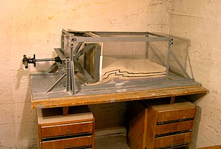
Analogue modelling is a laboratory experimental method using uncomplicated physical models with certain simple scales of time and length to model geological scenarios and simulate geodynamic evolutions.

References

  1. 1 2 "Stampede Charges Computational Science Forward in Tackling Complex Societal Challenges".
  2. 1 2 3 4 5 6 7 8 9 10 11 12 13 14 15 16 17 18 19 20 21 22 23 24 25 26 27 28 29 30 31 32 33 34 35 36 37 38 39 40 41 42 43 44 45 46 47 48 49 50 51 52 53 54 55 56 57 58 59 60 61 62 63 64 65 66 67 68 Ismail-Zadeh, A.; Tackley, P. (2010). Computational methods for geodynamics. Cambridge University Press.
  3. 1 2 3 4 5 6 7 8 9 10 11 12 Jing, L. (2003). "A review of techniques, advances and outstanding issues in numerical modelling for rock mechanics and rock engineering". International Journal of Rock Mechanics and Mining Sciences. 40 (3): 283–353. doi:10.1016/s1365-1609(03)00013-3.
  4. Koyi, H. (1997-04-01). "Analogue Modelling: From a Qualitative to a Quantitative Technique — a Historical Outline". Journal of Petroleum Geology. 20 (2): 223–238. Bibcode:1997JPetG..20..223K. doi:10.1111/j.1747-5457.1997.tb00774.x. ISSN   1747-5457. S2CID   128619258.
  5. 1 2 Barnichon, J. D. (1998). "Finite element modelling in structural and petroleum geology" (PDF).{{cite journal}}: Cite journal requires |journal= (help)
  6. Malavieille, J. (1984). "Modélisation expérimentale des chevauchements imbriqués : application aux chaines de montagnes". Bulletin de la Société Géologique de France. XXVI (1): 129–138. doi:10.2113/gssgfbull.S7-XXVI.1.129.
  7. Zhong, S.; Yuen, D. A.; Moresi, L. N.; Schubert, G (2007). "Numerical methods for mantle convection". Treatise in Geophysics. Bibcode:2007mady.book..227Z.
  8. PARRISH, D.K. (1973). "A non-linear finite element fold model". American Journal of Science. 273 (4): 318–334. Bibcode:1973AmJS..273..318P. doi:10.2475/ajs.273.4.318. hdl: 1911/14887 .
  9. De Bremaecker, J. -Cl.; Becker, Eric B. (1978-10-10). "Finite element models of folding". Tectonophysics. 50 (2): 349–367. Bibcode:1978Tectp..50..349D. doi:10.1016/0040-1951(78)90142-7.
  10. Turcotte, D. L.; Torrance, K. E.; Hsui, A. T. (1973). "Convection in the earth's mantle". Methods in Computational Physics. Methods in Computational Physics: Advances in Research and Applications. Vol. 13. New York: Academic Press. pp. 431–454. Bibcode:1973mcpr...13..431T. doi:10.1016/B978-0-12-460813-9.50016-3. ISBN   9780124608139.
  11. Ranalli, Giorgio (2001). "Experimental tectonics: from Sir James Hall to the present". Journal of Geodynamics. 32 (1–2): 65–76. Bibcode:2001JGeo...32...65R. doi:10.1016/s0264-3707(01)00023-0.
  12. 1 2 Computational Methods for Fluid Dynamics | Joel H. Ferziger | Springer. Springer. 2002. ISBN   9783540420743.
  13. Polyanin, Andrei; Schiesser, William; Zhurov, Alexei (2008-10-10). "Partial differential equation". Scholarpedia. 3 (10): 4605. Bibcode:2008SchpJ...3.4605P. doi: 10.4249/scholarpedia.4605 . ISSN   1941-6016.
  14. 1 2 3 Batchelor, G. K. (2000-02-28). An Introduction to Fluid Dynamics. Cambridge University Press. ISBN   9780521663960.
  15. Ghosh, Somnath; Kikuchi, Noboru (1991). "An arbitrary Lagrangian-Eulerian finite element method for large deformation analysis of elastic-viscoplastic solids". Computer Methods in Applied Mechanics and Engineering. 86 (2): 127–188. Bibcode:1991CMAME..86..127G. doi:10.1016/0045-7825(91)90126-q. hdl: 2027.42/29426 .
  16. 1 2 Hu, Y.; Randolph, M. F. (1998-05-01). "A practical numerical approach for large deformation problems in soil". International Journal for Numerical and Analytical Methods in Geomechanics. 22 (5): 327–350. Bibcode:1998IJNAM..22..327H. doi:10.1002/(sici)1096-9853(199805)22:5<327::aid-nag920>3.0.co;2-x. ISSN   1096-9853.
  17. 1 2 3 4 Taras., Gerya (2010). Introduction to numerical geodynamic modelling. Cambridge, UK: Cambridge University Press. ISBN   9780521887540. OCLC   664028049.
  18. Atkinson, Kendall (2007-08-29). "Numerical analysis". Scholarpedia. 2 (8): 3163. Bibcode:2007SchpJ...2.3163A. doi: 10.4249/scholarpedia.3163 . ISSN   1941-6016.
  19. 1 2 3 4 5 6 Jing, L.; Hudson, J. A. (2002-06-01). "Numerical methods in rock mechanics". International Journal of Rock Mechanics and Mining Sciences. Numerical Methods in Rock Mechanics. 39 (4): 409–427. doi:10.1016/S1365-1609(02)00065-5.
  20. 1 2 Oden, J. (2010-05-20). "Finite element method". Scholarpedia. 5 (5): 9836. Bibcode:2010SchpJ...5.9836O. doi: 10.4249/scholarpedia.9836 . ISSN   1941-6016.
  21. 1 2 3 4 5 6 7 8 9 10 11 12 13 Logan, Daryl L. (2016-01-01). A First Course in the Finite Element Method. Cengage Learning. ISBN   9781305635111.
  22. 1 2 3 4 5 Boyd, John P. (2001-12-03). Chebyshev and Fourier Spectral Methods: Second Revised Edition. Courier Corporation. ISBN   9780486411835.
  23. 1 2 3 4 5 Gottlieb, David; Gottlieb, Sigal (2009-09-02). "Spectral methods". Scholarpedia. 4 (9): 7504. Bibcode:2009SchpJ...4.7504G. doi: 10.4249/scholarpedia.7504 . ISSN   1941-6016.
  24. 1 2 3 Eymard, Robert; Gallouët, Thierry; Herbin, Raphaèle (2000-01-01). "Finite volume methods" (PDF). Handbook of Numerical Analysis. Solution of Equation in ℝ (Part 3), Techniques of Scientific Computing (Part 3). Vol. 7. Elsevier. pp. 713–1018. doi:10.1016/S1570-8659(00)07005-8. ISBN   9780444503503.
  25. 1 2 Eymard, Robert; Gallouët, Thierry; Herbin (2010-06-23). "Finite volume method". Scholarpedia. 5 (6): 9835. Bibcode:2010SchpJ...5.9835E. doi: 10.4249/scholarpedia.9835 . ISSN   1941-6016.
  26. Fornberg, Bengt (2011-10-19). "Finite difference method". Scholarpedia. 6 (10): 9685. Bibcode:2011SchpJ...6.9685F. doi: 10.4249/scholarpedia.9685 . ISSN   1941-6016.
  27. Numerical Treatment of Partial Differential Equations | Christian Grossmann | Springer. Universitext. Springer. 2007. ISBN   9783540715825.
  28. "D. Matrix Powers and Exponentials". Finite Difference Methods for Ordinary and Partial Differential Equations. Other Titles in Applied Mathematics. Society for Industrial and Applied Mathematics. 2007-01-01. pp. 285–310. doi:10.1137/1.9780898717839.appd. ISBN   9780898716290.
  29. Morton, K. W.; Mayers, D. F. (2005-04-11). Numerical Solution of Partial Differential Equations: An Introduction. Cambridge University Press. ISBN   9781139443203.
  30. 1 2 3 4 Smith, Gordon D. (1985). Numerical Solution of Partial Differential Equations: Finite Difference Methods. Clarendon Press. ISBN   9780198596509.
  31. CUNDALL, P. A. (1971). "A computer model for simulating progressive, large scale movement in blocky rock systems". Symp. ISRM, Nancy, France, Proc. 2: 129–136.
  32. Cundall, P. A. (2001-01-01). "A discontinuous future for numerical modelling in geomechanics?". Proceedings of the Institution of Civil Engineers - Geotechnical Engineering. 149 (1): 41–47. doi:10.1680/geng.2001.149.1.41. ISSN   1353-2618.
  33. Potyondy, D. O.; Cundall, P. A. (2004-12-01). "A bonded-particle model for rock". International Journal of Rock Mechanics and Mining Sciences. Rock Mechanics Results from the Underground Research Laboratory, Canada. 41 (8): 1329–1364. doi:10.1016/j.ijrmms.2004.09.011. S2CID   131601997.
  34. Zhang, Xiao-Ping; Wong, Louis Ngai Yuen (2013-09-01). "Crack Initiation, Propagation and Coalescence in Rock-Like Material Containing Two Flaws: a Numerical Study Based on Bonded-Particle Model Approach". Rock Mechanics and Rock Engineering. 46 (5): 1001–1021. Bibcode:2013RMRE...46.1001Z. doi:10.1007/s00603-012-0323-1. ISSN   0723-2632. S2CID   129821946.
  35. 1 2 Zhang, Xiao-Ping; Wong, Louis Ngai Yuen (2012-09-01). "Cracking Processes in Rock-Like Material Containing a Single Flaw Under Uniaxial Compression: A Numerical Study Based on Parallel Bonded-Particle Model Approach". Rock Mechanics and Rock Engineering. 45 (5): 711–737. Bibcode:2012RMRE...45..711Z. doi:10.1007/s00603-011-0176-z. ISSN   0723-2632. S2CID   140699474.
  36. Cardenas, IC (2023). "A two-dimensional approach to quantify stratigraphic uncertainty from borehole data using non-homogeneous random fields". Engineering Geology. 314: 107001. doi:10.1016/j.enggeo.2023.107001. S2CID   255634245.
  37. 1 2 3 4 Harrison, John P. (2001-01-26). Engineering Rock Mechanics: Part 2: Illustrative Worked Examples. Elsevier. ISBN   9780080530932.
  38. "Quartz: Quartz mineral information and data". www.mindat.org. Retrieved 2017-11-17.
  39. "Feldspar Group: Feldspar Group mineral information and data". www.mindat.org. Retrieved 2017-11-17.
  40. Wu, Zhijun; Wong, Louis Ngai Yuen (2012). "Frictional crack initiation and propagation analysis using the numerical manifold method". Computers and Geotechnics. 39: 38–53. doi:10.1016/j.compgeo.2011.08.011.
  41. 1 2 3 4 Braun, Jean; van der Beek, Peter; Valla, Pierre; Robert, Xavier; Herman, Frédéric; Glotzbach, Christoph; Pedersen, Vivi; Perry, Claire; Simon-Labric, Thibaud (2012-02-20). "Quantifying rates of landscape evolution and tectonic processes by thermochronology and numerical modeling of crustal heat transport using PECUBE". Tectonophysics. 524 (Supplement C): 1–28. Bibcode:2012Tectp.524....1B. doi:10.1016/j.tecto.2011.12.035.
  42. 1 2 Reiners, Peter W.; Ehlers, Todd A.; Zeitler, Peter K. (2005-01-01). "Past, Present, and Future of Thermochronology". Reviews in Mineralogy and Geochemistry. 58 (1): 1–18. Bibcode:2005RvMG...58....1R. doi:10.2138/rmg.2005.58.1. ISSN   1529-6466.
  43. 1 2 3 4 5 Braun, Jean (2003-07-01). "Pecube: a new finite-element code to solve the 3D heat transport equation including the effects of a time-varying, finite amplitude surface topography". Computers & Geosciences. 29 (6): 787–794. Bibcode:2003CG.....29..787B. doi:10.1016/S0098-3004(03)00052-9.
  44. 1 2 Braun, Jean; Beek, Peter van der; Valla, Pierre; Robert, Xavier; Herman, Frédéric; Glotzbach, Christoph; Pedersen, Vivi; Perry, Claire; Simon-Labric, Thibaud (2012). "Quantifying rates of landscape evolution and tectonic processes by thermochronology and numerical modeling of crustal heat transport using PECUBE". Tectonophysics. 524–525: 1–28. Bibcode:2012Tectp.524....1B. doi:10.1016/j.tecto.2011.12.035.
  45. Coutand, Isabelle; Whipp, David M.; Grujic, Djordje; Bernet, Matthias; Fellin, Maria Giuditta; Bookhagen, Bodo; Landry, Kyle R.; Ghalley, S. K.; Duncan, Chris (2014-02-01). "Geometry and kinematics of the Main Himalayan Thrust and Neogene crustal exhumation in the Bhutanese Himalaya derived from inversion of multithermochronologic data". Journal of Geophysical Research: Solid Earth. 119 (2): 2013JB010891. Bibcode:2014JGRB..119.1446C. doi: 10.1002/2013JB010891 . ISSN   2169-9356.
  46. Diersch, Hans-Jörg G. (2013-11-22). FEFLOW: Finite Element Modeling of Flow, Mass and Heat Transport in Porous and Fractured Media. Springer Science & Business Media. ISBN   9783642387395.
  47. Huyakorn, Peter S. (2012-12-02). Computational Methods in Subsurface Flow. Academic Press. ISBN   9780323137973.
  48. Pinder, George F.; Gray, William G. (2013-09-03). Finite Element Simulation in Surface and Subsurface Hydrology. Elsevier. ISBN   9781483270425.
  49. Irwin., Remson; M., Hornberger, George; J., Molz, Fred (1971). "Numerical methods in subsurface hydrology". AGRIS: International Information System for the Agricultural Science and Technology.
  50. Pinder, George F.; Gray, William G. (1976-02-01). "Is there a difference in the finite element method?". Water Resources Research. 12 (1): 105–107. Bibcode:1976WRR....12..105P. doi:10.1029/WR012i001p00105. ISSN   1944-7973.
  51. Anderson, Mary P.; Woessner, William W.; Hunt, Randall J. (2015-08-13). Applied Groundwater Modeling: Simulation of Flow and Advective Transport. Academic Press. ISBN   9780080916385.
  52. 1 2 3 4 5 6 7 Groundwater, USGS – U.S. Geological Survey Office of. "Information for New MODFLOW Users". water.usgs.gov. Retrieved 2017-10-12.
  53. McDonald, Michael G.; Harbaugh, Arlen W.; the original authors of MODFLOW (2003-03-01). "The History of MODFLOW". Ground Water. 41 (2): 280–283. doi:10.1111/j.1745-6584.2003.tb02591.x. ISSN   1745-6584. PMID   12656294. S2CID   21781355.
  54. 1 2 3 4 5 6 7 Zuo, Xuran; Chan, Lung Sang; Gao, Jian-Feng (2017-02-09). "Compression-extension transition of continental crust in a subduction zone: A parametric numerical modeling study with implications on Mesozoic-Cenozoic tectonic evolution of the Cathaysia Block". PLOS ONE. 12 (2): e0171536. Bibcode:2017PLoSO..1271536Z. doi: 10.1371/journal.pone.0171536 . ISSN   1932-6203. PMC   5300286 . PMID   28182640.
  55. Liao, Jie; Gerya, Taras; Thielmann, Marcel; Webb, A. Alexander G.; Kufner, Sofia-Katerina; Yin, An (2017). "3D geodynamic models for the development of opposing continental subduction zones: The Hindu Kush–Pamir example". Earth and Planetary Science Letters. 480: 133–146. Bibcode:2017E&PSL.480..133L. doi:10.1016/j.epsl.2017.10.005.
  56. Cundall, P. A. (1989-03-01). "Numerical experiments on localization in frictional materials". Ingenieur-Archiv. 59 (2): 148–159. doi:10.1007/BF00538368. ISSN   0020-1154. S2CID   118155529.
  57. Poliakov, A. N. B; van Balen, R; Podladchikov, Yu; Daudre, B; Cloetingh, S; Talbot, C (1993-11-15). "Numerical analysis of how sedimentation and redistribution of surficial sediments affects salt diapirism". Tectonophysics. The origin of sedimentary basins: Inferences from quantitative modelling and basin analysis. 226 (1): 199–216. Bibcode:1993Tectp.226..199P. doi:10.1016/0040-1951(93)90118-4.
  58. Poliakov, A. N. B.; Podladchikov, Yu.; Talbot, C. (1993-12-30). "Initiation of salt diapirs with frictional overburdens: numerical experiments". Tectonophysics. 228 (3): 199–210. Bibcode:1993Tectp.228..199P. doi:10.1016/0040-1951(93)90341-G.
  59. Poliakov, A. N. B.; Cundall, P. A.; Podladchikov, Y. Y.; Lyakhovsky, V. A. (1993). Flow and Creep in the Solar System: Observations, Modeling and Theory. NATO ASI Series. Springer, Dordrecht. pp. 175–195. doi:10.1007/978-94-015-8206-3_12. ISBN   9789048142453.
  60. Sobolev, S. V.; Petrunin, A.; Garfunkel, Z.; Babeyko, A. Y. (2005-09-30). "Thermo-mechanical model of the Dead Sea Transform". Earth and Planetary Science Letters. 238 (1): 78–95. Bibcode:2005E&PSL.238...78S. doi:10.1016/j.epsl.2005.06.058.
  61. Choi, Eun-seo; Lavier, Luc; Gurnis, Michael (2008-12-01). "Thermomechanics of mid-ocean ridge segmentation". Physics of the Earth and Planetary Interiors. Recent Advances in Computational Geodynamics: Theory, Numerics and Applications. 171 (1): 374–386. Bibcode:2008PEPI..171..374C. doi:10.1016/j.pepi.2008.08.010.
  62. Wang, Yuejun; Zhang, Feifei; Fan, Weiming; Zhang, Guowei; Chen, Shiyue; Cawood, Peter A.; Zhang, Aimei (2010-12-01). "Tectonic setting of the South China Block in the early Paleozoic: Resolving intracontinental and ocean closure models from detrital zircon U-Pb geochronology". Tectonics. 29 (6): TC6020. Bibcode:2010Tecto..29.6020W. doi: 10.1029/2010TC002750 . ISSN   1944-9194.
  63. 1 2 3 Wolfgang, Bangerth; Juliane, Dannberg; Rene, Gassmoeller; Timo, Heister; others (2017-04-12). "ASPECT: Advanced Solver for Problems in Earth's ConvecTion, User Manual". Figshare. doi:10.6084/m9.figshare.4865333.
  64. Kronbichler, Martin; Heister, Timo; Bangerth, Wolfgang (2012-10-01). "High accuracy mantle convection simulation through modern numerical methods" (PDF). Geophysical Journal International. 191 (1): 12–29. Bibcode:2012GeoJI.191...12K. doi:10.1111/j.1365-246x.2012.05609.x. ISSN   0956-540X.
  65. Stadler, Georg; Gurnis, Michael; Burstedde, Carsten; Wilcox, Lucas C.; Alisic, Laura; Ghattas, Omar (2010-08-27). "The Dynamics of Plate Tectonics and Mantle Flow: From Local to Global Scales". Science. 329 (5995): 1033–1038. Bibcode:2010Sci...329.1033S. doi:10.1126/science.1191223. ISSN   0036-8075. PMID   20798311. S2CID   23875605.
  66. 1 2 Gerya, Taras V.; Yuen, David A. (2003-12-30). "Characteristics-based marker-in-cell method with conservative finite-differences schemes for modeling geological flows with strongly variable transport properties". Physics of the Earth and Planetary Interiors. 140 (4): 293–318. Bibcode:2003PEPI..140..293G. doi:10.1016/j.pepi.2003.09.006.
  67. 1 2 Blankenbach, B.; Busse, F.; Christensen, U.; Cserepes, L.; Gunkel, D.; Hansen, U.; Harder, H.; Jarvis, G.; Koch, M. (1989-07-01). "A benchmark comparison for mantle convection codes". Geophysical Journal International. 98 (1): 23–38. Bibcode:1989GeoJI..98...23B. doi: 10.1111/j.1365-246X.1989.tb05511.x . ISSN   1365-246X.
  68. Travis, B. J.; Anderson, C.; Baumgardner, J.; Gable, C. W.; Hager, B. H.; O'Connell, R. J.; Olson, P.; Raefsky, A.; Schubert, G. (1990-12-01). "A benchmark comparison of numerical methods for infinite Prandtl number thermal convection in two-dimensional Cartesian geometry". Geophysical & Astrophysical Fluid Dynamics. 55 (3–4): 137–160. Bibcode:1990GApFD..55..137T. doi:10.1080/03091929008204111. ISSN   0309-1929.
  69. Busse, F. H.; Christensen, U.; Clever, R.; Cserepes, L.; Gable, C.; Giannandrea, E.; Guillou, L.; Houseman, G.; Nataf, H. C. (1994-08-01). "3D convection at infinite Prandtl number in Cartesian geometry — a benchmark comparison". Geophysical & Astrophysical Fluid Dynamics. 75 (1): 39–59. Bibcode:1994GApFD..75...39B. doi:10.1080/03091929408203646. ISSN   0309-1929.
  70. Stemmer, K.; Harder, H.; Hansen, U. (2006-08-31). "A new method to simulate convection with strongly temperature- and pressure-dependent viscosity in a spherical shell: Applications to the Earth's mantle". Physics of the Earth and Planetary Interiors. 157 (3): 223–249. Bibcode:2006PEPI..157..223S. doi:10.1016/j.pepi.2006.04.007.
  71. van Keken, P. E.; King, S. D.; Schmeling, H.; Christensen, U. R.; Neumeister, D.; Doin, M.-P. (1997-10-10). "A comparison of methods for the modeling of thermochemical convection". Journal of Geophysical Research: Solid Earth. 102 (B10): 22477–22495. Bibcode:1997JGR...10222477V. doi: 10.1029/97JB01353 . ISSN   2156-2202.
  72. Tackley, Paul J.; King, Scott D. (2003-04-01). "Testing the tracer ratio method for modeling active compositional fields in mantle convection simulations". Geochemistry, Geophysics, Geosystems. 4 (4): 8302. Bibcode:2003GGG.....4.8302T. doi: 10.1029/2001GC000214 . ISSN   1525-2027.
  73. Davies, D. R.; Davies, J. H.; Hassan, O.; Morgan, K.; Nithiarasu, P. (2007-05-01). "Investigations into the applicability of adaptive finite element methods to two-dimensional infinite Prandtl number thermal and thermochemical convection" (PDF). Geochemistry, Geophysics, Geosystems. 8 (5): Q05010. Bibcode:2007GGG.....8.5010D. doi:10.1029/2006GC001470. ISSN   1525-2027. S2CID   15080657.
  74. Larsen, Tine B.; Yuen, David A.; Moser, Jiří; Fornberg, Bengt (1997-04-01). "A high-order finite-difference method applied to large Rayleigh number mantle convection". Geophysical & Astrophysical Fluid Dynamics. 84 (1–2): 53–83. Bibcode:1997GApFD..84...53L. doi:10.1080/03091929708208973. ISSN   0309-1929.
  75. Trompert, R. A.; Hansen, U. (1996-12-01). "The application of a finite volume multigrid method to three-dimensional flow problems in a highly viscous fluid with a variable viscosity". Geophysical & Astrophysical Fluid Dynamics. 83 (3–4): 261–291. Bibcode:1996GApFD..83..261T. doi:10.1080/03091929608208968. ISSN   0309-1929.
  76. Auth, C.; Harder, H. (1999-06-01). "Multigrid solution of convection problems with strongly variable viscosity". Geophysical Journal International. 137 (3): 793–804. Bibcode:1999GeoJI.137..793A. doi: 10.1046/j.1365-246x.1999.00833.x . ISSN   0956-540X.
  77. Albers, Michael (2000-05-01). "A Local Mesh Refinement Multigrid Method for 3-D Convection Problems with Strongly Variable Viscosity". Journal of Computational Physics. 160 (1): 126–150. Bibcode:2000JCoPh.160..126A. doi:10.1006/jcph.2000.6438.
  78. Kameyama, Masanori; Kageyama, Akira; Sato, Tetsuya (2005-06-10). "Multigrid iterative algorithm using pseudo-compressibility for three-dimensional mantle convection with strongly variable viscosity". Journal of Computational Physics. 206 (1): 162–181. arXiv: physics/0410249 . Bibcode:2005JCoPh.206..162K. doi:10.1016/j.jcp.2004.11.030. S2CID   15776061.
  79. Gerya, Taras V.; Yuen, David A. (2007-08-15). "Robust characteristics method for modelling multiphase visco-elasto-plastic thermo-mechanical problems". Physics of the Earth and Planetary Interiors. Computational Challenges in the Earth Sciences. 163 (1): 83–105. Bibcode:2007PEPI..163...83G. doi:10.1016/j.pepi.2007.04.015.
  80. Choblet, Gaël (2005-05-01). "Modelling thermal convection with large viscosity gradients in one block of the 'cubed sphere'". Journal of Computational Physics. 205 (1): 269–291. Bibcode:2005JCoPh.205..269C. doi:10.1016/j.jcp.2004.11.005.
  81. Hernlund, John W.; Tackley, Paul J. (2008-12-01). "Modeling mantle convection in the spherical annulus". Physics of the Earth and Planetary Interiors. Recent Advances in Computational Geodynamics: Theory, Numerics and Applications. 171 (1): 48–54. Bibcode:2008PEPI..171...48H. doi:10.1016/j.pepi.2008.07.037.
  82. Kageyama, Akira; Sato, Tetsuya (2004-09-01). ""Yin-Yang grid": An overset grid in spherical geometry". Geochemistry, Geophysics, Geosystems (Submitted manuscript). 5 (9): Q09005. arXiv: physics/0403123 . Bibcode:2004GGG.....5.9005K. doi:10.1029/2004GC000734. ISSN   1525-2027. S2CID   119434182.
  83. Kameyama, Masanori; Kageyama, Akira; Sato, Tetsuya (2008). "Multigrid-based simulation code for mantle convection in spherical shell using Yin–Yang grid". Physics of the Earth and Planetary Interiors. 171 (1–4): 19–32. Bibcode:2008PEPI..171...19K. doi:10.1016/j.pepi.2008.06.025.
  84. Tackley, Paul J. (2008). "Modelling compressible mantle convection with large viscosity contrasts in a three-dimensional spherical shell using the yin-yang grid". Physics of the Earth and Planetary Interiors. 171 (1–4): 7–18. Bibcode:2008PEPI..171....7T. doi:10.1016/j.pepi.2008.08.005.
  85. Hüttig, Christian; Stemmer, Kai (2008-02-01). "The spiral grid: A new approach to discretize the sphere and its application to mantle convection". Geochemistry, Geophysics, Geosystems. 9 (2): Q02018. Bibcode:2008GGG.....9.2018H. doi: 10.1029/2007GC001581 . ISSN   1525-2027.
  86. "Computational Infrastructure for Geodynamics :: Software". geodynamics.org.
  87. King, Scott D.; Raefsky, Arthur; Hager, Bradford H. (1990-01-01). "Conman: vectorizing a finite element code for incompressible two-dimensional convection in the Earth's mantle". Physics of the Earth and Planetary Interiors. 59 (3): 195–207. Bibcode:1990PEPI...59..195K. doi:10.1016/0031-9201(90)90225-M.
  88. Moresi, L.‐N.; Solomatov, V. S. (1995-09-01). "Numerical investigation of 2D convection with extremely large viscosity variations". Physics of Fluids. 7 (9): 2154–2162. Bibcode:1995PhFl....7.2154M. doi:10.1063/1.868465. ISSN   1070-6631.
  89. Moresi, Louis; Gurnis, Michael (1996-02-01). "Constraints on the lateral strength of slabs from three-dimensional dynamic flow models". Earth and Planetary Science Letters. 138 (1): 15–28. Bibcode:1996E&PSL.138...15M. doi:10.1016/0012-821X(95)00221-W.
  90. Frick, H.; Busse, F. H.; Clever, R. M. (1983-02-01). "Steady three-dimensional convection at high Prandtl numbers". Journal of Fluid Mechanics. 127: 141–153. Bibcode:1983JFM...127..141F. doi:10.1017/S0022112083002669. ISSN   0022-1120. S2CID   123109920.
  91. Cserepes, L.; Rabinowicz, M.; Rosemberg-Borot, C. (1988-10-10). "Three-dimensional infinite Prandtl number convection in one and two layers with implications for the Earth's gravity field". Journal of Geophysical Research: Solid Earth. 93 (B10): 12009–12025. Bibcode:1988JGR....9312009C. doi:10.1029/JB093iB10p12009. ISSN   2156-2202.
  92. Gable, Carl W.; O'Connell, Richard J.; Travis, Bryan J. (1991-05-10). "Convection in three dimensions with surface plates: Generation of toroidal flow". Journal of Geophysical Research: Solid Earth. 96 (B5): 8391–8405. Bibcode:1991JGR....96.8391G. doi:10.1029/90JB02743. ISSN   2156-2202.
  93. Young, Richard E. (1974). "Finite-amplitude thermal convection in a spherical shell". Journal of Fluid Mechanics. 63 (4): 695–721. Bibcode:1974JFM....63..695Y. doi:10.1017/S0022112074002151. ISSN   1469-7645. S2CID   122193142.
  94. Glatzmaier, Gary A. (1988-12-01). "Numerical simulations of mantle convection: Time-dependent, three-dimensional, compressible, spherical shell". Geophysical & Astrophysical Fluid Dynamics. 43 (2): 223–264. Bibcode:1988GApFD..43..223G. doi:10.1080/03091928808213626. ISSN   0309-1929. S2CID   121395950.
  95. Monnereau, Marc; Quéré, Sandrine (2001-01-30). "Spherical shell models of mantle convection with tectonic plates". Earth and Planetary Science Letters. 184 (3): 575–587. Bibcode:2001E&PSL.184..575M. doi:10.1016/S0012-821X(00)00334-4.
  96. Monnereau, Marc; Quéré, Sandrine (2001). "Spherical shell models of mantle convection with tectonic plates". Earth and Planetary Science Letters. 184 (3–4): 575–587. Bibcode:2001E&PSL.184..575M. doi:10.1016/s0012-821x(00)00334-4.
  97. C., Condie, Kent (1997). Plate tectonics and crustal evolution. Condie, Kent C. (4th ed.). Oxford: Butterworth Heinemann. ISBN   9780750633864. OCLC   174141325.
  98. Christensen, U.R.; Wicht, J. (2015). Treatise on Geophysics. pp. 245–277. doi:10.1016/b978-0-444-53802-4.00145-7. ISBN   9780444538031.
  99. 1 2 Christensen, U.R.; Aubert, J.; Cardin, P.; Dormy, E.; Gibbons, S.; Glatzmaier, G.A.; Grote, E.; Honkura, Y.; Jones, C. (2001). "A numerical dynamo benchmark". Physics of the Earth and Planetary Interiors. 128 (1–4): 25–34. Bibcode:2001PEPI..128...25C. doi:10.1016/s0031-9201(01)00275-8.
  100. Glatzmaier, Gary A.; Roberts, Paul H. (1995). "A three-dimensional convective dynamo solution with rotating and finitely conducting inner core and mantle". Physics of the Earth and Planetary Interiors. 91 (1–3): 63–75. Bibcode:1995PEPI...91...63G. doi:10.1016/0031-9201(95)03049-3.
  101. Soward, Andrew M. (2002-11-28). Magnetohydrodynamics and the Earth's Core: Selected Works by Paul Roberts. CRC Press. ISBN   9780415272223.
  102. Kageyama, Akira; Sato, Tetsuya (1995-05-01). "Computer simulation of a magnetohydrodynamic dynamo. II". Physics of Plasmas. 2 (5): 1421–1431. Bibcode:1995PhPl....2.1421K. doi:10.1063/1.871485. ISSN   1070-664X.
  103. Helmut, Harder; Ulrich, Hansen (2005-05-01). "A finite-volume solution method for thermal convection and dynamo problems in spherical shells". Geophysical Journal International. 161 (2): 522. Bibcode:2005GeoJI.161..522H. doi: 10.1111/j.1365-246X.2005.02560.x . ISSN   0956-540X.
  104. Chan, Kit H.; Zhang, Keke; Li, Ligang; Liao, Xinhao (2007). "A new generation of convection-driven spherical dynamos using EBE finite element method". Physics of the Earth and Planetary Interiors. 163 (1–4): 251–265. Bibcode:2007PEPI..163..251C. doi:10.1016/j.pepi.2007.04.017.
  105. "Geodynamo". websites.pmc.ucsc.edu. Retrieved 2017-10-13.
  106. 1 2 3 Komatitsch, Dimitri; Vilotte, Jean-Pierre (1998-04-01). "The spectral element method: An efficient tool to simulate the seismic response of 2D and 3D geological structures". Bulletin of the Seismological Society of America. 88 (2): 368–392. doi:10.1785/BSSA0880020368. ISSN   0037-1106. S2CID   123800174.
  107. Virieux, J. (1986-04-01). "P-SV wave propagation in heterogeneous media: Velocity‐stress finite‐difference method". Geophysics. 51 (4): 889–901. Bibcode:1986Geop...51..889V. doi:10.1190/1.1442147. ISSN   0016-8033.
  108. Bohlen, Thomas (2002). "Parallel 3-D viscoelastic finite difference seismic modelling". Computers & Geosciences. 28 (8): 887–899. Bibcode:2002CG.....28..887B. doi:10.1016/s0098-3004(02)00006-7.
  109. Javaherian, Abdolrahim (1994-08-01). "Grid dispersion in generating finite-differences synthetic seismograms". Acta Seismologica Sinica. 7 (3): 397–407. Bibcode:1994AcSSn...7..397J. doi:10.1007/BF02650677. ISSN   1000-9116. S2CID   108702596.
  110. Komatitsch, Dimitri; Tromp, Jeroen (2002-07-01). "Spectral-element simulations of global seismic wave propagation—II. Three-dimensional models, oceans, rotation and self-gravitation". Geophysical Journal International. 150 (1): 303–318. Bibcode:2002GeoJI.150..303K. doi: 10.1046/j.1365-246X.2002.01716.x . ISSN   0956-540X.
  111. Rudolph, Maxwell L.; Lekić, Vedran; Lithgow-Bertelloni, Carolina (2015-12-11). "Viscosity jump in Earth's mid-mantle". Science. 350 (6266): 1349–1352. Bibcode:2015Sci...350.1349R. doi: 10.1126/science.aad1929 . ISSN   0036-8075. PMID   26659053. S2CID   1448877.
  112. Stead, D.; Eberhardt, E.; Coggan, J.S. (2006). "Developments in the characterization of complex rock slope deformation and failure using numerical modelling techniques". Engineering Geology. 83 (1–3): 217–235. doi:10.1016/j.enggeo.2005.06.033.