Part of a series on |
Linguistics |
---|
Portal |
Analogical modeling (AM) is a formal theory of exemplar based analogical reasoning, proposed by Royal Skousen, professor of Linguistics and English language at Brigham Young University in Provo, Utah. It is applicable to language modeling and other categorization tasks. Analogical modeling is related to connectionism and nearest neighbor approaches, in that it is data-based rather than abstraction-based; but it is distinguished by its ability to cope with imperfect datasets (such as caused by simulated short term memory limits) and to base predictions on all relevant segments of the dataset, whether near or far. In language modeling, AM has successfully predicted empirically valid forms for which no theoretical explanation was known (see the discussion of Finnish morphology in Skousen et al. 2002).
An exemplar-based model consists of a general-purpose modeling engine and a problem-specific dataset. Within the dataset, each exemplar (a case to be reasoned from, or an informative past experience) appears as a feature vector: a row of values for the set of parameters that define the problem. For example, in a spelling-to-sound task, the feature vector might consist of the letters of a word. Each exemplar in the dataset is stored with an outcome, such as a phoneme or phone to be generated. When the model is presented with a novel situation (in the form of an outcome-less feature vector), the engine algorithmically sorts the dataset to find exemplars that helpfully resemble it, and selects one, whose outcome is the model's prediction. The particulars of the algorithm distinguish one exemplar-based modeling system from another.
In AM, we think of the feature values as characterizing a context, and the outcome as a behavior that occurs within that context. Accordingly, the novel situation is known as the given context. Given the known features of the context, the AM engine systematically generates all contexts that include it (all of its supracontexts), and extracts from the dataset the exemplars that belong to each. The engine then discards those supracontexts whose outcomes are inconsistent (this measure of consistency will be discussed further below), leaving an analogical set of supracontexts, and probabilistically selects an exemplar from the analogical set with a bias toward those in large supracontexts. This multilevel search exponentially magnifies the likelihood of a behavior's being predicted as it occurs reliably in settings that specifically resemble the given context.
AM performs the same process for each case it is asked to evaluate. The given context, consisting of n variables, is used as a template to generate supracontexts. Each supracontext is a set of exemplars in which one or more variables have the same values that they do in the given context, and the other variables are ignored. In effect, each is a view of the data, created by filtering for some criteria of similarity to the given context, and the total set of supracontexts exhausts all such views. Alternatively, each supracontext is a theory of the task or a proposed rule whose predictive power needs to be evaluated.
It is important to note that the supracontexts are not equal peers one with another; they are arranged by their distance from the given context, forming a hierarchy. If a supracontext specifies all of the variables that another one does and more, it is a subcontext of that other one, and it lies closer to the given context. (The hierarchy is not strictly branching; each supracontext can itself be a subcontext of several others, and can have several subcontexts.) This hierarchy becomes significant in the next step of the algorithm.
The engine now chooses the analogical set from among the supracontexts. A supracontext may contain exemplars that only exhibit one behavior; it is deterministically homogeneous and is included. It is a view of the data that displays regularity, or a relevant theory that has never yet been disproven. A supracontext may exhibit several behaviors, but contain no exemplars that occur in any more specific supracontext (that is, in any of its subcontexts); in this case it is non-deterministically homogeneous and is included. Here there is no great evidence that a systematic behavior occurs, but also no counterargument. Finally, a supracontext may be heterogeneous, meaning that it exhibits behaviors that are found in a subcontext (closer to the given context), and also behaviors that are not. Where the ambiguous behavior of the nondeterministically homogeneous supracontext was accepted, this is rejected because the intervening subcontext demonstrates that there is a better theory to be found. The heterogeneous supracontext is therefore excluded. This guarantees that we see an increase in meaningfully consistent behavior in the analogical set as we approach the given context.
With the analogical set chosen, each appearance of an exemplar (for a given exemplar may appear in several of the analogical supracontexts) is given a pointer to every other appearance of an exemplar within its supracontexts. One of these pointers is then selected at random and followed, and the exemplar to which it points provides the outcome. This gives each supracontext an importance proportional to the square of its size, and makes each exemplar likely to be selected in direct proportion to the sum of the sizes of all analogically consistent supracontexts in which it appears. Then, of course, the probability of predicting a particular outcome is proportional to the summed probabilities of all the exemplars that support it.
(Skousen 2002, in Skousen et al. 2002, pp. 11–25, and Skousen 2003, both passim)
Given a context with elements:
This terminology is best understood through an example. In the example used in the second chapter of Skousen (1989), each context consists of three variables with potential values 0-3
The two outcomes for the dataset are e and r, and the exemplars are:
3 1 0 e 0 3 2 r 2 1 0 r 2 1 2 r 3 1 1 r
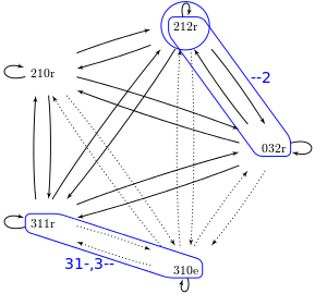
We define a network of pointers like so:
The solid lines represent pointers between exemplars with matching outcomes; the dotted lines represent pointers between exemplars with non-matching outcomes.
The statistics for this example are as follows:
Behavior can only be predicted for a given context; in this example, let us predict the outcome for the context "3 1 2". To do this, we first find all of the contexts containing the given context; these contexts are called supracontexts. We find the supracontexts by systematically eliminating the variables in the given context; with m variables, there will generally be supracontexts. The following table lists each of the sub- and supracontexts; x means "not x", and - means "anything".
Supracontext | Subcontexts |
---|---|
3 1 2 | 3 1 2 |
3 1 - | 3 1 2, 3 1 2 |
3 - 2 | 3 1 2, 3 1 2 |
- 1 2 | 3 1 2, 3 1 2 |
3 - - | 3 1 2, 3 1 2, 3 1 2, 3 12 |
- 1 - | 3 1 2, 3 1 2, 3 1 2, 3 1 2 |
- - 2 | 3 1 2, 3 1 2, 3 1 2, 31 2 |
- - - | 3 1 2, 3 1 2, 3 1 2, 3 1 2, 31 2, 3 1 2, 3 12, 312 |
These contexts are shown in the venn diagram below:
The next step is to determine which exemplars belong to which contexts in order to determine which of the contexts are homogeneous. The table below shows each of the subcontexts, their behavior in terms of the given exemplars, and the number of disagreements within the behavior:
Subcontext | Behavior | Disagreements |
---|---|---|
3 1 2 | (empty) | 0 |
3 1 2 | 3 1 0 e, 3 1 1 r | 2 |
3 1 2 | (empty) | 0 |
3 1 2 | 2 1 2 r | 0 |
3 12 | (empty) | 0 |
3 1 2 | 2 1 0 r | 0 |
31 2 | 0 3 2 r | 0 |
312 | (empty) | 0 |
Analyzing the subcontexts in the table above, we see that there is only 1 subcontext with any disagreements: "3 1 2", which in the dataset consists of "3 1 0 e" and "3 1 1 r". There are 2 disagreements in this subcontext; 1 pointing from each of the exemplars to the other (see the pointer network pictured above). Therefore, only supracontexts containing this subcontext will contain any disagreements. We use a simple rule to identify the homogeneous supracontexts:
If the number if disagreements in the supracontext is greater than the number of disagreements in the contained subcontext, we say that it is heterogeneous; otherwise, it is homogeneous.
There are 3 situations that produce a homogeneous supracontext:
The only two heterogeneous supracontexts are "- 1 -" and "- - -". In both of them, it is the combination of the non-deterministic "3 1 2" with other subcontexts containing the r outcome which causes the heterogeneity.
There is actually a 4th type of homogeneous supracontext: it contains more than one non-empty subcontext and it is non-deterministic, but the frequency of outcomes in each sub-context is exactly the same. Analogical modeling does not consider this situation, however, for 2 reasons:
Next we construct the analogical set, which consists of all of the pointers and outcomes from the homogeneous supracontexts. The figure below shows the pointer network with the homogeneous contexts highlighted.
The pointers are summarized in the following table:
Homogeneous supracontext | Occurrences | Number of pointers | ||
---|---|---|---|---|
| ||||
3 1 - | "3 1 0 e", "3 1 1 r" |
| ||
- 1 2 | "2 1 2 r" |
| ||
3 - - | "3 1 0 e", "3 1 1 r" |
| ||
- - 2 | "2 1 2 r", "0 3 2 r" |
| ||
Totals: |
|
4 of the pointers in the analogical set are associated with the outcome e, and the other 9 are associated with r. In AM, a pointer is randomly selected and the outcome it points to is predicted. With a total of 13 pointers, the probability of the outcome e being predicted is 4/13 or 30.8%, and for outcome r it is 9/13 or 69.2%. We can create a more detailed account by listing the pointers for each of the occurrences in the homogeneous supracontexts:
Occurrence | Number of homogeneous supracontexts | Number of pointers | Analogical effect |
---|---|---|---|
3 1 0 e | 2 | 4 | 30.8% |
3 1 1 r | 2 | 4 | 30.8% |
2 1 2 r | 2 | 3 | 23.1% |
0 3 2 r | 1 | 2 | 15.4% |
2 1 0 r | 0 | 0 | 0.0% |
We can then see the analogical effect of each of the instances in the data set.
Analogy has been considered useful in describing language at least since the time of Saussure. Noam Chomsky and others have more recently criticized analogy as too vague to really be useful (Bańko 1991), an appeal to a deus ex machina. Skousen's proposal appears to address that criticism by proposing an explicit mechanism for analogy, which can be tested for psychological validity.
Analogical modeling has been employed in experiments ranging from phonology and morphology (linguistics) to orthography and syntax.
Though analogical modeling aims to create a model free from rules seen as contrived by linguists, in its current form it still requires researchers to select which variables to take into consideration. This is necessary because of the so-called "exponential explosion" of processing power requirements of the computer software used to implement analogical modeling. Recent research suggests that quantum computing could provide the solution to such performance bottlenecks (Skousen et al. 2002, see pp 45–47).
A mathematical model is an abstract description of a concrete system using mathematical concepts and language. The process of developing a mathematical model is termed mathematical modeling. Mathematical models are used in applied mathematics and in the natural sciences and engineering disciplines, as well as in non-physical systems such as the social sciences (such as economics, psychology, sociology, political science). It can also be taught as a subject in its own right.
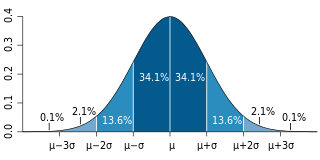
Probability theory or probability calculus is the branch of mathematics concerned with probability. Although there are several different probability interpretations, probability theory treats the concept in a rigorous mathematical manner by expressing it through a set of axioms. Typically these axioms formalise probability in terms of a probability space, which assigns a measure taking values between 0 and 1, termed the probability measure, to a set of outcomes called the sample space. Any specified subset of the sample space is called an event.
In probability theory and statistics, a probability distribution is the mathematical function that gives the probabilities of occurrence of different possible outcomes for an experiment. It is a mathematical description of a random phenomenon in terms of its sample space and the probabilities of events.
A statistical model is a mathematical model that embodies a set of statistical assumptions concerning the generation of sample data. A statistical model represents, often in considerably idealized form, the data-generating process. When referring specifically to probabilities, the corresponding term is probabilistic model.
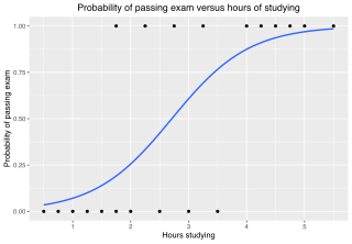
In statistics, the logistic model is a statistical model that models the log-odds of an event as a linear combination of one or more independent variables. In regression analysis, logistic regression is estimating the parameters of a logistic model. Formally, in binary logistic regression there is a single binary dependent variable, coded by an indicator variable, where the two values are labeled "0" and "1", while the independent variables can each be a binary variable or a continuous variable. The corresponding probability of the value labeled "1" can vary between 0 and 1, hence the labeling; the function that converts log-odds to probability is the logistic function, hence the name. The unit of measurement for the log-odds scale is called a logit, from logistic unit, hence the alternative names. See § Background and § Definition for formal mathematics, and § Example for a worked example.
In philosophy of mind and cognitive science, folk psychology, or commonsense psychology, is a human capacity to explain and predict the behavior and mental state of other people. Processes and items encountered in daily life such as pain, pleasure, excitement, and anxiety use common linguistic terms as opposed to technical or scientific jargon. Folk psychology allows for an insight into social interactions and communication, thus stretching the importance of connection and how it is experienced.
Cross-validation, sometimes called rotation estimation or out-of-sample testing, is any of various similar model validation techniques for assessing how the results of a statistical analysis will generalize to an independent data set. Cross-validation includes resampling and sample splitting methods that use different portions of the data to test and train a model on different iterations. It is often used in settings where the goal is prediction, and one wants to estimate how accurately a predictive model will perform in practice. It can also be used to assess the quality of a fitted model and the stability of its parameters.
In the field of mathematical optimization, stochastic programming is a framework for modeling optimization problems that involve uncertainty. A stochastic program is an optimization problem in which some or all problem parameters are uncertain, but follow known probability distributions. This framework contrasts with deterministic optimization, in which all problem parameters are assumed to be known exactly. The goal of stochastic programming is to find a decision which both optimizes some criteria chosen by the decision maker, and appropriately accounts for the uncertainty of the problem parameters. Because many real-world decisions involve uncertainty, stochastic programming has found applications in a broad range of areas ranging from finance to transportation to energy optimization.
In statistics, the coefficient of determination, denoted R2 or r2 and pronounced "R squared", is the proportion of the variation in the dependent variable that is predictable from the independent variable(s).
In statistics, ordinary least squares (OLS) is a type of linear least squares method for choosing the unknown parameters in a linear regression model by the principle of least squares: minimizing the sum of the squares of the differences between the observed dependent variable in the input dataset and the output of the (linear) function of the independent variable.
This glossary of statistics and probability is a list of definitions of terms and concepts used in the mathematical sciences of statistics and probability, their sub-disciplines, and related fields. For additional related terms, see Glossary of mathematics and Glossary of experimental design.
In statistics, Poisson regression is a generalized linear model form of regression analysis used to model count data and contingency tables. Poisson regression assumes the response variable Y has a Poisson distribution, and assumes the logarithm of its expected value can be modeled by a linear combination of unknown parameters. A Poisson regression model is sometimes known as a log-linear model, especially when used to model contingency tables.
In information theory, perplexity is a measure of uncertainty in the value of a sample from a discrete probability distribution. The larger the perplexity, the less likely it is that an observer can guess the value which will be drawn from the distribution. Perplexity was originally introduced in 1977 in the context of speech recognition by Frederick Jelinek, Robert Leroy Mercer, Lalit R. Bahl, and James K. Baker.
In statistics, Mallows's, named for Colin Lingwood Mallows, is used to assess the fit of a regression model that has been estimated using ordinary least squares. It is applied in the context of model selection, where a number of predictor variables are available for predicting some outcome, and the goal is to find the best model involving a subset of these predictors. A small value of means that the model is relatively precise.
In cybernetics, the term variety denotes the total number of distinguishable elements of a set, most often the set of states, inputs, or outputs of a finite-state machine or transformation, or the binary logarithm of the same quantity. Variety is used in cybernetics as an information theory that is easily related to deterministic finite automata, and less formally as a conceptual tool for thinking about organization, regulation, and stability. It is an early theory of complexity in automata, complex systems, and operations research.
In statistics, least-angle regression (LARS) is an algorithm for fitting linear regression models to high-dimensional data, developed by Bradley Efron, Trevor Hastie, Iain Johnstone and Robert Tibshirani.
In the statistical analysis of observational data, propensity score matching (PSM) is a statistical matching technique that attempts to estimate the effect of a treatment, policy, or other intervention by accounting for the covariates that predict receiving the treatment. PSM attempts to reduce the bias due to confounding variables that could be found in an estimate of the treatment effect obtained from simply comparing outcomes among units that received the treatment versus those that did not. Paul R. Rosenbaum and Donald Rubin introduced the technique in 1983.
In statistics, multivariate adaptive regression splines (MARS) is a form of regression analysis introduced by Jerome H. Friedman in 1991. It is a non-parametric regression technique and can be seen as an extension of linear models that automatically models nonlinearities and interactions between variables.
In quantum physics, a quantum state is a mathematical entity that embodies the knowledge of a quantum system. Quantum mechanics specifies the construction, evolution, and measurement of a quantum state. The result is a quantum-mechanical prediction for the system represented by the state. Knowledge of the quantum state, and the quantum mechanical rules for the system's evolution in time, exhausts all that can be known about a quantum system.
Fairness in machine learning refers to the various attempts at correcting algorithmic bias in automated decision processes based on machine learning models. Decisions made by computers after a machine-learning process may be considered unfair if they were based on variables considered sensitive. For example gender, ethnicity, sexual orientation or disability. As it is the case with many ethical concepts, definitions of fairness and bias are always controversial. In general, fairness and bias are considered relevant when the decision process impacts people's lives. In machine learning, the problem of algorithmic bias is well known and well studied. Outcomes may be skewed by a range of factors and thus might be considered unfair with respect to certain groups or individuals. An example would be the way social media sites deliver personalized news to consumers.