Direct-quadrature-zero transformation

"Odq" redirects here. For other uses, see ODQ (disambiguation).

The direct-quadrature-zero (DQZ, DQ0 ^[1] or DQO, ^[2] sometimes lowercase) or Parktransformation (named after Robert H. Park) is a tensor that rotates the reference frame of a three-element vector or a three-by-three element matrix in an effort to simplify analysis. The transformation is equivalent to the product of the Clarke transformation and a rotation ^[3] .

The Park transformation is often used in the context of electrical engineering with three-phase circuits. The transformation can be used to rotate the reference frames of AC waveforms such that they become DC signals. Simplified calculations can then be carried out on these DC quantities before performing the inverse transformation to recover the actual three-phase AC results. As an example, the Park transformation is often used in order to simplify the analysis of three-phase synchronous machines or to simplify calculations for the control of three-phase inverters. In analysis of three-phase synchronous machines, the transformation transfers three-phase stator and rotor quantities into a single rotating reference frame to eliminate the effect of time-varying inductances and transformation the system into a linear time-invariant system

Introduction

The Park transformation is equivalent to the product of the rotation and Clarke transformation matrices. The Clarke transformation (named after Edith Clarke) converts vectors in the ABC reference frame to the XYZ (also called αβγ) reference frame. The primary value of the Clarke transformation is isolating that part of the ABC-referenced vector, which is common to all three components of the vector; it isolates the common-mode component (i.e., the Z component). The power-invariant, right-handed, uniformly-scaled Clarke transformation matrix is

${\displaystyle K_{C}={\sqrt {\frac {2}{3}}}\cdot {\begin{bmatrix}1&-{\frac {1}{2}}&-{\frac {1}{2}}\\0&{\frac {\sqrt {3}}{2}}&-{\frac {\sqrt {3}}{2}}\\{\frac {1}{\sqrt {2}}}&{\frac {1}{\sqrt {2}}}&{\frac {1}{\sqrt {2}}}\end{bmatrix}}}$.

To convert an ABC-referenced column vector to the XYZ reference frame, the vector must be pre-multiplied by the Clarke transformation matrix:

${\displaystyle {\vec {u}}_{XYZ}=K_{C}\cdot {\vec {u}}_{ABC}}$.

And, to convert back from an XYZ-referenced column vector to the ABC reference frame, the vector must be pre-multiplied by the inverse Clarke transformation matrix:

${\displaystyle {\vec {u}}_{ABC}=K_{C}^{-1}\cdot {\vec {u}}_{XYZ}}$.

The rotation converts vectors in the XYZ reference frame to the DQZ reference frame. The rotation's primary value is to rotate a vector's reference frame at an arbitrary frequency. The rotation shifts the signal's frequency spectrum such that the arbitrary frequency now appears as "dc," and the old dc appears as the negative of the arbitrary frequency. The rotation matrix is

${\displaystyle K_{r}={\begin{bmatrix}\cos {\left(\theta \right)}&\sin {\left(\theta \right)}&0\\-\sin {\left(\theta \right)}&\cos {\left(\theta \right)}&0\\0&0&1\end{bmatrix}}}$,

where θ is the instantaneous angle of an arbitrary ω frequency. To convert an XYZ-referenced vector to the DQZ reference frame, the column vector signal must be pre-multiplied by the rotation matrix:

${\displaystyle u_{P}=K_{r}\cdot u_{XYZ}}$.

And, to convert back from a DQZ-referenced vector to the XYZ reference frame, the column vector signal must be pre-multiplied by the inverse rotation matrix:

${\displaystyle u_{XYZ}=K_{r}^{-1}\cdot u_{DQZ}}$.

The Park transformation is equivalent to the product of the Clarke transformation and a rotation:

${\displaystyle K_{P}=K_{r}\cdot K_{C}}$

${\displaystyle \to {\begin{bmatrix}\cos {\left(\theta \right)}&\sin {\left(\theta \right)}&0\\-\sin {\left(\theta \right)}&\cos {\left(\theta \right)}&0\\0&0&1\end{bmatrix}}\cdot {\sqrt {\frac {2}{3}}}{\begin{bmatrix}1&{\frac {-1}{2}}&{\frac {-1}{2}}\\0&{\frac {\sqrt {3}}{2}}&-{\frac {\sqrt {3}}{2}}\\{\frac {1}{\sqrt {2}}}&{\frac {1}{\sqrt {2}}}&{\frac {1}{\sqrt {2}}}\end{bmatrix}}}$

${\displaystyle \to {\sqrt {\frac {2}{3}}}{\begin{bmatrix}\cos {\left(\theta \right)}&\cos {\left(\theta -{\frac {2\pi }{3}}\right)}&\cos {\left(\theta +{\frac {2\pi }{3}}\right)}\\-\sin {\left(\theta \right)}&-\sin {\left(\theta -{\frac {2\pi }{3}}\right)}&-\sin {\left(\theta +{\frac {2\pi }{3}}\right)}\\{\frac {\sqrt {2}}{2}}&{\frac {\sqrt {2}}{2}}&{\frac {\sqrt {2}}{2}}\end{bmatrix}}}$

The inverse transformation is:

${\displaystyle K_{P}^{-1}={\sqrt {\frac {2}{3}}}{\begin{bmatrix}\cos {\left(\theta \right)}&-\sin {\left(\theta \right)}&{\frac {\sqrt {2}}{2}}\\\cos {\left(\theta -{\frac {2\pi }{3}}\right)}&-\sin {\left(\theta -{\frac {2\pi }{3}}\right)}&{\frac {\sqrt {2}}{2}}\\\cos {\left(\theta +{\frac {2\pi }{3}}\right)}&-\sin {\left(\theta +{\frac {2\pi }{3}}\right)}&{\frac {\sqrt {2}}{2}}\end{bmatrix}}}$

To convert an ABC-referenced vector to the DQZ reference frame, the column vector signal must be pre-multiplied by the Park transformation matrix:

${\displaystyle u_{DQZ}=K_{P}\cdot u_{ABC}}$.

And, to convert back from a DQZ-referenced vector to the ABC reference frame, the column vector signal must be pre-multiplied by the inverse Park transformation matrix:

${\displaystyle u_{ABC}=K_{P}^{-1}\cdot u_{DQZ}}$.

To understand this transformation better, a derivation of the transformation is included.

Derivation

Rotation matrix derivation

A rotation matrix is based on the concept of the dot product and projections of vectors onto other vectors. First, let us imagine two unit vectors, ${\displaystyle {\hat {u}}_{D}}$ and ${\displaystyle {\hat {u}}_{Q}}$ (the unit vectors, or axes, of the new reference frame from the perspective of the old reference frame), and a third, arbitrary, vector ${\displaystyle {\vec {v}}_{XY}}$. We can define the two unit vectors and the random vector in terms of their Cartesian coordinates in the old reference frame:

${\displaystyle {\hat {u}}_{D}=\cos {\left(\theta \right)}{\hat {u}}_{X}+\sin {\left(\theta \right)}{\hat {u}}_{Y}}$

${\displaystyle {\hat {u}}_{Q}=-\sin {\left(\theta \right)}{\hat {u}}_{X}+\cos {\left(\theta \right)}{\hat {u}}_{Y}}$

${\displaystyle {\vec {v}}_{XY}=v_{X}{\hat {u}}_{X}+v_{Y}{\hat {u}}_{Y}}$,

where ${\displaystyle {\hat {u}}_{X}}$ and ${\displaystyle {\hat {u}}_{Y}}$ are the unit basis vectors of the old coordinate system and ${\displaystyle \theta }$ is the angle between the ${\displaystyle {\hat {u}}_{X}}$ and ${\displaystyle {\hat {u}}_{D}}$ unit vectors (i.e., the angle between the two reference frames). The projection of the arbitrary vector onto each of the two new unit vectors implies the dot product:

${\displaystyle v_{D}={\hat {u}}_{D}\cdot {\vec {v}}_{XY}}$

${\displaystyle \to \cos {\left(\theta \right)}v_{X}+\sin {\left(\theta \right)}v_{Y}}$

${\displaystyle v_{Q}={\hat {u}}_{Q}\cdot {\vec {v}}_{XY}}$

${\displaystyle \to -\sin {\left(\theta \right)}v_{X}+\cos {\left(\theta \right)}v_{Y}}$.

So, ${\displaystyle v_{D}}$ is the projection of ${\displaystyle {\vec {v}}_{XY}}$ onto the ${\displaystyle {\hat {u}}_{D}}$ axis, and ${\displaystyle v_{Q}}$ is the projection of ${\displaystyle {\vec {v}}_{XY}}$ onto the ${\displaystyle {\hat {u}}_{Q}}$ axis. These new vector components, ${\displaystyle v_{D}}$ and ${\displaystyle v_{Q}}$, together compose the new vector ${\displaystyle {\vec {v}}_{DQ}}$, the original vector ${\displaystyle {\vec {v}}_{XY}}$ in terms of the new DQ reference frame.

Projection of ${\displaystyle {\vec {v}}_{XY}}$ onto the DQ reference frame.

Notice that the positive angle ${\displaystyle \theta }$ above caused the arbitrary vector to rotate backward when transitioned to the new DQ reference frame. In other words, its angle concerning the new reference frame is less than its angle to the old reference frame. This is because the reference frame, not the vector, was rotated forwards. Actually, a forward rotation of the reference frame is identical to a negative rotation of the vector. If the old reference frame were rotating forwards, such as in three-phase electrical systems, then the resulting DQ vector remains stationary.

A single matrix equation can summarize the operation above:

${\displaystyle {\vec {v}}_{DQ}={\begin{bmatrix}\cos {\left(\theta \right)}&\sin {\left(\theta \right)}\\-\sin {\left(\theta \right)}&\cos {\left(\theta \right)}\end{bmatrix}}\cdot {\vec {v}}_{XY}}$.

This tensor can be expanded to three-dimensional problems, where the axis about which rotation occurs is left unaffected. In the following example, the rotation is about the Z axis, but any axis could have been chosen:

${\displaystyle K_{r}={\begin{bmatrix}\cos {\left(\theta \right)}&\sin {\left(\theta \right)}&0\\-\sin {\left(\theta \right)}&\cos {\left(\theta \right)}&0\\0&0&1\end{bmatrix}}}$.

From a linear algebra perspective, this is simply a clockwise rotation about the z-axis and is mathematically equivalent to the trigonometric difference angle formulae.

Clarke transformation derivation

The ABC unit basis vectors

Consider a three-dimensional space with unit basis vectors A, B, and C. The sphere in the figure below is used to show the scale of the reference frame for context and the box is used to provide a rotational context.

ABC unit basis vectors.

Typically, in electrical engineering (or any other context that uses three-phase systems), the three-phase components are shown in a two-dimensional perspective. However, given the three phases can change independently, they are by definition orthogonal to each other. This implies a three-dimensional perspective, as shown in the figure above. So, the two-dimensional perspective is really showing the projection of the three-dimensional reality onto a plane.

Two-dimensional perspective of a three-dimensional reality.

Three-phase problems are typically described as operating within this plane. In reality, the problem is likely a balanced-phase problem (i.e., v_A + v_B + v_C = 0) and the net vector

${\displaystyle {\vec {v}}=v_{A}{\hat {u}}_{A}+v_{B}{\hat {u}}_{B}+v_{C}{\hat {u}}_{C}}$

is always on this plane.

The AYC' unit basis vectors

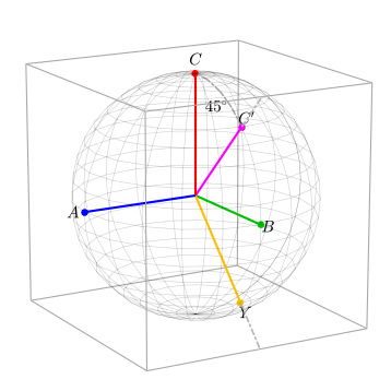
To build the Clarke transformation, we actually use the Park transformation in two steps. Our goal is to rotate the C axis into the corner of the box. This way the rotated C axis will be orthogonal to the plane of the two-dimensional perspective mentioned above. The first step towards building the Clarke transformation requires rotating the ABC reference frame about the A axis. So, this time, the 1 will be in the first element of the Park transformation:

${\displaystyle K_{1}={\begin{bmatrix}1&0&0\\0&\cos {\left(-{\frac {\pi }{4}}\right)}&\sin {\left(-{\frac {\pi }{4}}\right)}\\0&-\sin {\left(-{\frac {\pi }{4}}\right)}&\cos {\left(-{\frac {\pi }{4}}\right)}\end{bmatrix}}}$

${\displaystyle \to {\begin{bmatrix}1&0&0\\0&{\frac {1}{\sqrt {2}}}&-{\frac {1}{\sqrt {2}}}\\0&{\frac {1}{\sqrt {2}}}&{\frac {1}{\sqrt {2}}}\end{bmatrix}}}$

The following figure shows how the ABC reference frame is rotated to the AYC' reference frame when any vector is pre-multiplied by the K₁ matrix. The C' and Y axes now point to the midpoints of the edges of the box, but the magnitude of the reference frame has not changed (i.e., the sphere did not grow or shrink).This is due to the fact that the norm of the K₁ tensor is 1: ||K₁|| = 1. This means that any vector in the ABC reference frame will continue to have the same magnitude when rotated into the AYC' reference frame.

AYC' unit basis vectors. The C' and Y axes now point to the edges of the box, but the magnitude has not changed.

The XYZ unit basis vectors

Next, the following tensor rotates the vector about the new Y axis in a counter-clockwise direction with respect to the Y axis (The angle was chosen so that the C' axis would be pointed towards the corner of the box.):

${\displaystyle K_{2}={\begin{bmatrix}\cos {\left(\theta \right)}&0&-\sin {\left(\theta \right)}\\0&1&0\\\sin {\left(\theta \right)}&0&\cos {\left(\theta \right)}\end{bmatrix}}}$

${\displaystyle \theta =\cos ^{-1}\left({\sqrt {\frac {2}{3}}}\right)\to 35.26^{\circ }}$,

or

${\displaystyle K_{2}={\begin{bmatrix}{\sqrt {\frac {2}{3}}}&0&-{\frac {1}{\sqrt {3}}}\\0&1&0\\{\frac {1}{\sqrt {3}}}&0&{\sqrt {\frac {2}{3}}}\end{bmatrix}}}$.

Notice that the distance from the center of the sphere to the midpoint of the edge of the box is √2 but from the center of the sphere to the corner of the box is √3. That is where the 35.26° angle came from. The angle can be calculated using the dot product. Let ${\displaystyle {\vec {m}}=\left(0,{\frac {\sqrt {2}}{2}},{\frac {\sqrt {2}}{2}}\right)}$ be the unit vector in the direction of C' and let ${\displaystyle {\vec {n}}=\left({\frac {1}{\sqrt {3}}},{\frac {1}{\sqrt {3}}},{\frac {1}{\sqrt {3}}}\right)}$ be a unit vector in the direction of the corner of the box at ${\displaystyle {\vec {n}}=\left(1,1,1\right)}$. Because ${\displaystyle {\vec {m}}\cdot {\vec {n}}=|{\vec {m}}||{\vec {n}}|\cos \theta ,}$ where ${\displaystyle \theta }$ is the angle between ${\displaystyle {\vec {m}}}$ and ${\displaystyle {\vec {n}},}$ we have

${\displaystyle \left(0,{\frac {\sqrt {2}}{2}},{\frac {\sqrt {2}}{2}}\right)\cdot \left({\frac {1}{\sqrt {3}}},{\frac {1}{\sqrt {3}}},{\frac {1}{\sqrt {3}}}\right)=\cos \theta }$

${\displaystyle \cos \theta =0+{\frac {\sqrt {2}}{2{\sqrt {3}}}}+{\frac {\sqrt {2}}{2{\sqrt {3}}}}={\sqrt {\frac {2}{3}}}}$

${\displaystyle \theta =\cos ^{-1}\left({\sqrt {\frac {2}{3}}}\right)}$

${\displaystyle \theta =35.26^{\circ }.}$

The norm of the K₂ matrix is also 1, so it too does not change the magnitude of any vector pre-multiplied by the K₂ matrix.

XYZ unit basis vectors. The Z axis (rotated C' axis) now points into the corner of the box.

The zero plane

At this point, the Z axis is now orthogonal to the plane in which any ABC vector without a common-mode component can be found. Any balanced ABC vector waveform (a vector without a common mode) will travel about this plane. This plane will be called the zero plane and is shown below by the hexagonal outline.

Plane of the vectors without common mode indicated by the hexagonal outline. The Z axis is orthogonal to this plane, and the X axis is parallel to the projection of the A axis onto the zero plane.

The X and Y basis vectors are on the zero plane. Notice that the X axis is parallel to the projection of the A axis onto the zero plane. The X axis is slightly larger than the projection of the A axis onto the zero plane. It is larger by a factor of √3/2. The arbitrary vector did not change magnitude through this conversion from the ABC reference frame to the XYZ reference frame (i.e., the sphere did not change size). This is true for the power-invariant form of the Clarke transformation. The following figure shows the common two-dimensional perspective of the ABC and XYZ reference frames.

Two-dimensional perspective of the ABC and XYZ reference frames.

It might seem odd that though the magnitude of the vector did not change, the magnitude of its components did (i.e., the X and Y components are longer than the A, B, and C components). Perhaps this can be intuitively understood by considering that for a vector without common mode, what took three values (A, B, and C components) to express, now only takes 2 (X and Y components) since the Z component is zero. Therefore, the X and Y component values must be larger to compensate.

Combination of tensors

The power-invariant Clarke transformation matrix is a combination of the K₁ and K₂ tensors:

${\displaystyle K_{C}=\underbrace {\begin{bmatrix}{\sqrt {\frac {2}{3}}}&0&-{\frac {1}{\sqrt {3}}}\\0&1&0\\{\frac {1}{\sqrt {3}}}&0&{\sqrt {\frac {2}{3}}}\end{bmatrix}} _{K_{2}}\cdot \underbrace {\begin{bmatrix}1&0&0\\0&{\frac {1}{\sqrt {2}}}&-{\frac {1}{\sqrt {2}}}\\0&{\frac {1}{\sqrt {2}}}&{\frac {1}{\sqrt {2}}}\end{bmatrix}} _{K_{1}}}$,

or

${\displaystyle K_{C}={\sqrt {\frac {2}{3}}}\cdot {\begin{bmatrix}1&-{\frac {1}{2}}&-{\frac {1}{2}}\\0&{\frac {\sqrt {3}}{2}}&-{\frac {\sqrt {3}}{2}}\\{\frac {1}{\sqrt {2}}}&{\frac {1}{\sqrt {2}}}&{\frac {1}{\sqrt {2}}}\end{bmatrix}}}$

${\displaystyle \to {\begin{bmatrix}{\frac {2}{\sqrt {6}}}&-{\frac {1}{\sqrt {6}}}&-{\frac {1}{\sqrt {6}}}\\0&{\frac {1}{\sqrt {2}}}&-{\frac {1}{\sqrt {2}}}\\{\frac {1}{\sqrt {3}}}&{\frac {1}{\sqrt {3}}}&{\frac {1}{\sqrt {3}}}\end{bmatrix}}}$.

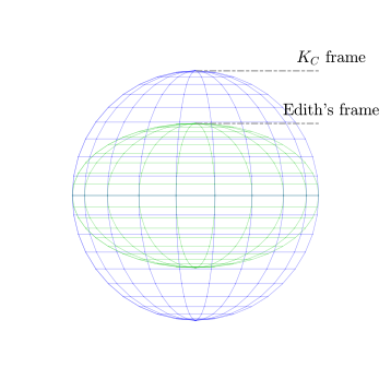
Notice that when multiplied through, the bottom row of the K_C matrix is 1/√3, not 1/3. (Edith Clarke did use 1/3 for the power-variant case.) The Z component is not exactly the average of the A, B, and C components. If only the bottom row elements were changed to be 1/3, then the sphere would be squashed along the Z axis. This means that the Z component would not have the same scaling as the X and Y components.

K_C frame (blue) and the original Edith matrix (green).

As things are written above, the norm of the Clarke transformation matrix is still 1, which means that it only rotates an ABC vector but does not scale it. The same cannot be said for Clarke's original transformation.

It is easy to verify (by matrix multiplication) that the inverse of K_C is

${\displaystyle K_{C}^{-1}={\begin{bmatrix}{\frac {2}{\sqrt {6}}}&0&{\frac {1}{\sqrt {3}}}\\-{\frac {1}{\sqrt {6}}}&{\frac {1}{\sqrt {2}}}&{\frac {1}{\sqrt {3}}}\\-{\frac {1}{\sqrt {6}}}&-{\frac {1}{\sqrt {2}}}&{\frac {1}{\sqrt {3}}}\end{bmatrix}}}$

Power-variant form

It is sometimes desirable to scale the Clarke transformation matrix so that the X axis is the projection of the A axis onto the zero plane. To do this, we uniformly apply a scaling factor of √2/3 and a ²√1/radical^{[ why? ]} to the zero component to get the power-variant Clarke transformation matrix:

${\displaystyle K_{\hat {C}}={\sqrt {\frac {2}{3}}}\cdot \underbrace {{\sqrt {\frac {2}{3}}}\cdot {\begin{bmatrix}1&-{\frac {1}{2}}&-{\frac {1}{2}}\\0&{\frac {\sqrt {3}}{2}}&-{\frac {\sqrt {3}}{2}}\\{\frac {1}{2}}&{\frac {1}{2}}&{\frac {1}{2}}\end{bmatrix}}} _{K_{C}}}$

${\displaystyle \to {\frac {2}{3}}{\begin{bmatrix}1&-{\frac {1}{2}}&-{\frac {1}{2}}\\0&{\frac {\sqrt {3}}{2}}&-{\frac {\sqrt {3}}{2}}\\{\frac {1}{2}}&{\frac {1}{2}}&{\frac {1}{2}}\end{bmatrix}}}$

or

${\displaystyle K_{\hat {C}}={\begin{bmatrix}{\frac {2}{3}}&-{\frac {1}{3}}&-{\frac {1}{3}}\\0&{\frac {1}{\sqrt {3}}}&-{\frac {1}{\sqrt {3}}}\\{\frac {1}{3}}&{\frac {1}{3}}&{\frac {1}{3}}\end{bmatrix}}}$.

This will necessarily shrink the sphere by a factor of √2/3 as shown below. Notice that this new X axis is exactly the projection of the A axis onto the zero plane.

The scaled XYZ reference frame of the power-variant Clarke transformation.

With the power-variant Clarke transformation, the magnitude of the arbitrary vector is smaller in the XYZ reference frame than in the ABC reference frame (the norm of the transformation is √2/3), but the magnitudes of the individual vector components are the same (when there is no common mode). So, as an example, a signal defined by

${\displaystyle {\begin{bmatrix}A\\B\\C\end{bmatrix}}={\begin{bmatrix}\cos {\left(\omega t\right)}\\\cos {\left(\omega t-{\frac {2\pi }{3}}\right)}\\\cos {\left(\omega t+{\frac {2\pi }{3}}\right)}\end{bmatrix}}}$

becomes, in the XYZ reference frame,

${\displaystyle {\begin{bmatrix}X\\Y\\Z\end{bmatrix}}={\begin{bmatrix}\cos {\left(\omega t\right)}\\\cos {\left(\omega t-{\frac {\pi }{2}}\right)}\\0\end{bmatrix}}}$,

a new vector whose components are the same magnitude as the original components: 1. In many cases, this is an advantageous quality of the power-variant Clarke transformation.

Park transformation derivation

The Park transformation is equivalent to applying the Clarke transformation to convert ABC-referenced vectors into two differential-mode components (i.e., X and Y) and one common-mode component (i.e., Z) and then a rotation to rotate the reference frame about the Z axis at some given angle. The X component becomes the D component, which is in direct alignment with the vector of rotation, and the Y component becomes the Q component, which is at a quadrature angle to the direct component. The Park transformation is

${\displaystyle K_{P}=K_{r}\cdot K_{C}}$

${\displaystyle \to {\begin{bmatrix}\cos {\left(\theta \right)}&\sin {\left(\theta \right)}&0\\-\sin {\left(\theta \right)}&\cos {\left(\theta \right)}&0\\0&0&1\end{bmatrix}}\cdot {\sqrt {\frac {2}{3}}}{\begin{bmatrix}1&{\frac {-1}{2}}&{\frac {-1}{2}}\\0&{\frac {\sqrt {3}}{2}}&-{\frac {\sqrt {3}}{2}}\\{\frac {1}{\sqrt {2}}}&{\frac {1}{\sqrt {2}}}&{\frac {1}{\sqrt {2}}}\end{bmatrix}}}$.

Example

In electric systems, very often the A, B, and C values are oscillating in such a way that the net vector is spinning. In a balanced system, the vector is spinning about the Z axis. Very often, it is helpful to rotate the reference frame such that the majority of the changes in the ABC values, due to this spinning, are canceled out and any finer variations become more obvious. This is incredibly useful as it now transforms the system into a linear time-invariant system.

The Park transformation can be thought of in geometric terms as the projection of the three separate sinusoidal phase quantities onto two axes rotating with the same angular velocity as the sinusoidal phase quantities.

DQZ example.

Shown above is the Park transformation as applied to the stator of a synchronous machine. There are three windings separated by 120 physical degrees. The three phase currents are equal in magnitude and are separated from one another by 120 electrical degrees. The three phase currents lag their corresponding phase voltages by ${\displaystyle \delta }$. The DQ axes are shown rotating with angular velocity equal to ${\displaystyle \omega }$, the same angular velocity as the phase voltages and currents. The D axis makes an angle ${\displaystyle \theta =\omega t}$ with the phase A winding which has been chosen as the reference. The currents ${\displaystyle I_{D}}$ and ${\displaystyle I_{Q}}$ are constant dc quantities.

Transformation originally proposed by Robert H. Park

The transformation originally proposed by Robert H. Park ^[4] differs slightly from the one given above. In such transformation, the q-axis is ahead of d-axis, qd0, and the ${\displaystyle \theta }$ angle is the angle between phase-a and d-axis, as given below. ^{[5] [6]}

${\displaystyle P={\frac {2}{3}}{\begin{bmatrix}\cos(\theta )&\cos(\theta -{\frac {2\pi }{3}})&\cos(\theta +{\frac {2\pi }{3}})\\-\sin(\theta )&-\sin(\theta -{\frac {2\pi }{3}})&-\sin(\theta +{\frac {2\pi }{3}})\\{\frac {1}{2}}&{\frac {1}{2}}&{\frac {1}{2}}\end{bmatrix}}}$

and

${\displaystyle P^{-1}={\begin{bmatrix}\cos(\theta )&-\sin(\theta )&1\\\cos(\theta -{\frac {2\pi }{3}})&-\sin(\theta -{\frac {2\pi }{3}})&1\\\cos(\theta +{\frac {2\pi }{3}})&-\sin(\theta +{\frac {2\pi }{3}})&1\end{bmatrix}}}$

References

In-line references

1. "Perform transformation from three-phase (abc) signal to dq0 rotating reference frame or the inverse". Simulink. 2018-09-27. Retrieved 2019-01-11.
2. Mihailovic, Zoran (1998-06-26). "Modeling and Control Design of Vsi-Fed Pmsm Drive Systems With Active Load" (PDF). ETDs. Retrieved 2019-01-11.
3. O’Rourke, Colm J.; Qasim, Mohammad M.; Overlin, Matthew R.; Kirtley, James L. (December 2019). "A Geometric Interpretation of Reference Frames and Transformations: dq0, Clarke, and Park". IEEE Transactions on Energy Conversion. 34 (4): 2070–2083. doi:10.1109/TEC.2019.2941175. ISSN   1558-0059.
4. Park, R. H. (July 1929). "Two-reaction theory of synchronous machines generalized method of analysis-part I". Transactions of the American Institute of Electrical Engineers. 48 (3): 716–727. doi:10.1109/T-AIEE.1929.5055275. ISSN   2330-9431.
5. D. Holmes and T. Lipo, "Pulse Width Modulation for Power Converters: Principles and Practice", Wiley-IEEE Press, 2003.
6. P. Krause, O. Wasynczuk and S. Sudhoff, "Analysis of Electric Machinery and Drive Systems", 2nd ed., Piscataway, NJ: IEEE Press, 2002.

General references

• C.J. O'Rourke et al. "A Geometric Interpretation of Reference Frames and Transformations: dq0, Clarke, and Park," in IEEE Transactions on Energy Conversion, vol. 34, no. 4, pp. 2070-2083, Dec. 2019.
• J. Lewis Blackburn Symmetrical Components for Power Systems Engineering, Marcel Dekker, New York (1993), ISBN   0-8247-8767-6.
• Zhang et al. A three-phase inverter with a neutral leg with space vector modulation IEEE APEC '97 Conference Proceedings (1997).
• T.A.Lipo, “A Cartesian Vector Approach To Reference Theory of AC Machines”, Int. Conference On Electric Machines, Laussane, Sept. 18–24, 1984.

See also

• Symmetrical components
• αβγ transformation
• Vector control (motor)