Linear separability

Last updated December 09, 2023

In Euclidean geometry, linear separability is a property of two sets of points. This is most easily visualized in two dimensions (the Euclidean plane) by thinking of one set of points as being colored blue and the other set of points as being colored red. These two sets are linearly separable if there exists at least one line in the plane with all of the blue points on one side of the line and all the red points on the other side. This idea immediately generalizes to higher-dimensional Euclidean spaces if the line is replaced by a hyperplane.

Mathematical definition

Let $X_{0}$ and $X_{1}$ be two sets of points in an n-dimensional Euclidean space. Then $X_{0}$ and $X_{1}$ are linearly separable if there exist n + 1 real numbers $w_{1},w_{2},..,w_{n},k$ , such that every point $x\in X_{0}$ satisfies $\sum _{i=1}^{n}w_{i}x_{i}>k$ and every point $x\in X_{1}$ satisfies $\sum _{i=1}^{n}w_{i}x_{i}<k$ , where $x_{i}$ is the $i$ -th component of $x$ .

Equivalently, two sets are linearly separable precisely when their respective convex hulls are disjoint (colloquially, do not overlap).^[1]

In simple 2D, it can also be imagined that the set of points under a linear transformation collapses into a line, on which there exists a value, k, greater than which one set of points will fall into, and lesser than which the other set of points fall.

Examples

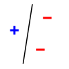
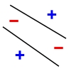
Three non-collinear points in two classes ('+' and '-') are always linearly separable in two dimensions. This is illustrated by the three examples in the following figure (the all '+' case is not shown, but is similar to the all '-' case):

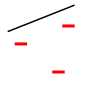
However, not all sets of four points, no three collinear, are linearly separable in two dimensions. The following example would need two straight lines and thus is not linearly separable:

Notice that three points which are collinear and of the form "+ ⋅⋅⋅ — ⋅⋅⋅ +" are also not linearly separable.

Number of linear separations

Let $T(N,K)$ be the number of ways to linearly separate N points (in general position) in K dimensions, then^[2]

T(N,K)=\left\{{\begin{array}{cc}2^{N}&K\geq N\\2\sum _{k=0}^{K-1}\left({\begin{array}{c}N-1\\k\end{array}}\right)&K<N\end{array}}\right.

When K is large, $T(N,K)/2^{N}$ is very close to one when $N\leq 2K$ , but very close to zero when $N>2K$ . In words, one perceptron unit can almost certainly memorize a random assignment of binary labels on N points when $N\leq 2K$ , but almost certainly not when $N>2K$ .

Linear separability of Boolean functions in n variables

A Boolean function in n variables can be thought of as an assignment of 0 or 1 to each vertex of a Boolean hypercube in n dimensions. This gives a natural division of the vertices into two sets. The Boolean function is said to be linearly separable provided these two sets of points are linearly separable. The number of distinct Boolean functions is $2^{2^{n}}$ where n is the number of variables passed into the function.^[3]

Such functions are also called linear threshold logic, or perceptrons. The classical theory is summarized in,^[4] as Knuth claims.^[5]

The value is only known exactly up to $n=9$ case, but the order of magnitude is known quite exactly: it has upper bound $2^{n^{2}-n\log _{2}n+O(n)}$ and lower bound $2^{n^{2}-n\log _{2}n-O(n)}$ .^[6]

It is co-NP-complete to decide whether a Boolean function given in disjunctive or conjunctive normal form is linearly separable.^[6]

Number of linearly separable Boolean functions in each dimension^[7](sequence A000609 in the OEIS )
Number of variables	Boolean functions	Linearly separable Boolean functions
2	16	14
3	256	104
4	65536	1882
5	4294967296	94572
6	18446744073709552000	15028134
7	3.402823669 ×10^38	8378070864
8	1.157920892 ×10^77	17561539552946
9	1.340780792 ×10^154	144130531453121108

Support vector machines

Classifying data is a common task in machine learning. Suppose some data points, each belonging to one of two sets, are given and we wish to create a model that will decide which set a new data point will be in. In the case of support vector machines, a data point is viewed as a p-dimensional vector (a list of p numbers), and we want to know whether we can separate such points with a (p − 1)-dimensional hyperplane. This is called a linear classifier. There are many hyperplanes that might classify (separate) the data. One reasonable choice as the best hyperplane is the one that represents the largest separation, or margin, between the two sets. So we choose the hyperplane so that the distance from it to the nearest data point on each side is maximized. If such a hyperplane exists, it is known as the maximum-margin hyperplane and the linear classifier it defines is known as a maximum margin classifier .

More formally, given some training data ${\mathcal {D}}$ , a set of n points of the form

{\mathcal {D}}=\left\{(\mathbf {x} _{i},y_{i})\mid \mathbf {x} _{i}\in \mathbb {R} ^{p},\,y_{i}\in \{-1,1\}\right\}_{i=1}^{n}

where the y_i is either 1 or −1, indicating the set to which the point $\mathbf {x} _{i}$ belongs. Each $\mathbf {x} _{i}$ is a p-dimensional real vector. We want to find the maximum-margin hyperplane that divides the points having $y_{i}=1$ from those having $y_{i}=-1$ . Any hyperplane can be written as the set of points $\mathbf {x}$ satisfying

\mathbf {w} \cdot \mathbf {x} -b=0,

where $\cdot$ denotes the dot product and ${\mathbf {w} }$ the (not necessarily normalized) normal vector to the hyperplane. The parameter ${\tfrac {b}{\|\mathbf {w} \|}}$ determines the offset of the hyperplane from the origin along the normal vector ${\mathbf {w} }$ .

If the training data are linearly separable, we can select two hyperplanes in such a way that they separate the data and there are no points between them, and then try to maximize their distance.

Related Research Articles

In mathematics and physics, a vector space is a set whose elements, often called vectors, may be added together and multiplied ("scaled") by numbers called scalars. Scalars are often real numbers, but can be complex numbers or, more generally, elements of any field. The operations of vector addition and scalar multiplication must satisfy certain requirements, called vector axioms. Real vector space and complex vector space are kinds of vector spaces based on different kinds of scalars: real coordinate space or complex coordinate space.

In Euclidean geometry, an affine transformation or affinity is a geometric transformation that preserves lines and parallelism, but not necessarily Euclidean distances and angles.

In machine learning, support vector machines are supervised learning models with associated learning algorithms that analyze data for classification and regression analysis. Developed at AT&T Bell Laboratories by Vladimir Vapnik with colleagues SVMs are one of the most robust prediction methods, being based on statistical learning frameworks or VC theory proposed by Vapnik and Chervonenkis (1974). Given a set of training examples, each marked as belonging to one of two categories, an SVM training algorithm builds a model that assigns new examples to one category or the other, making it a non-probabilistic binary linear classifier. SVM maps training examples to points in space so as to maximise the width of the gap between the two categories. New examples are then mapped into that same space and predicted to belong to a category based on which side of the gap they fall.

In the field of machine learning, the goal of statistical classification is to use an object's characteristics to identify which class it belongs to. A linear classifier achieves this by making a classification decision based on the value of a linear combination of the characteristics. An object's characteristics are also known as feature values and are typically presented to the machine in a vector called a feature vector. Such classifiers work well for practical problems such as document classification, and more generally for problems with many variables (features), reaching accuracy levels comparable to non-linear classifiers while taking less time to train and use. 5-12-23

In geometry, a hyperplane is a subspace whose dimension is one less than that of its ambient space. For example, if a space is 3-dimensional then its hyperplanes are the 2-dimensional planes, while if the space is 2-dimensional, its hyperplanes are the 1-dimensional lines. This notion can be used in any general space in which the concept of the dimension of a subspace is defined.

In machine learning, the perceptron is an algorithm for supervised learning of binary classifiers. A binary classifier is a function which can decide whether or not an input, represented by a vector of numbers, belongs to some specific class. It is a type of linear classifier, i.e. a classification algorithm that makes its predictions based on a linear predictor function combining a set of weights with the feature vector.

In geometry, a normal is an object that is perpendicular to a given object. For example, the normal line to a plane curve at a given point is the line perpendicular to the tangent line to the curve at the point.

<span class="mw-page-title-main">Projective space</span> Completion of the usual space with "points at infinity"

In mathematics, the concept of a projective space originated from the visual effect of perspective, where parallel lines seem to meet at infinity. A projective space may thus be viewed as the extension of a Euclidean space, or, more generally, an affine space with points at infinity, in such a way that there is one point at infinity of each direction of parallel lines.

In mathematics, an affine space is a geometric structure that generalizes some of the properties of Euclidean spaces in such a way that these are independent of the concepts of distance and measure of angles, keeping only the properties related to parallelism and ratio of lengths for parallel line segments. Affine space is the setting for affine geometry.

In projective geometry, duality or plane duality is a formalization of the striking symmetry of the roles played by points and lines in the definitions and theorems of projective planes. There are two approaches to the subject of duality, one through language and the other a more functional approach through special mappings. These are completely equivalent and either treatment has as its starting point the axiomatic version of the geometries under consideration. In the functional approach there is a map between related geometries that is called a duality. Such a map can be constructed in many ways. The concept of plane duality readily extends to space duality and beyond that to duality in any finite-dimensional projective geometry.

<span class="mw-page-title-main">Line (geometry)</span> Straight figure with zero width and depth

In geometry, a straight line, usually abbreviated line, is an infinitely long object with no width, depth, or curvature, an idealization of such physical objects as a straightedge, a taut string, or a ray of light. Lines are spaces of dimension one, which may be embedded in spaces of dimension two, three, or higher. The word line may also refer, in everyday life, to a line segment, which is a part of a line delimited by two points.

In mathematics, the real coordinate space or real coordinate n-space, of dimension $n$ , denoted $R n$ or , is the set of the $n$ -tuples of real numbers, that is the set of all sequences of $n$ real numbers. Special cases are called the real line $R 1$ , the real coordinate plane $R 2$ , and the real coordinate three-dimensional space $R 3$ . With component-wise addition and scalar multiplication, it is a real vector space, and its elements are called coordinate vectors.

In geometry, a set of points in space are coplanar if there exists a geometric plane that contains them all. For example, three points are always coplanar, and if the points are distinct and non-collinear, the plane they determine is unique. However, a set of four or more distinct points will, in general, not lie in a single plane.

In geometry, a three-dimensional space is a mathematical space in which three values (coordinates) are required to determine the position of a point. Most commonly, it is the three-dimensional Euclidean space, that is, the Euclidean space of dimension three, which models physical space. More general three-dimensional spaces are called 3-manifolds. The term may also refer colloquially to a subset of space, a three-dimensional region, a solid figure.

In machine learning, kernel machines are a class of algorithms for pattern analysis, whose best known member is the support-vector machine (SVM). These methods involve using linear classifiers to solve nonlinear problems. The general task of pattern analysis is to find and study general types of relations in datasets. For many algorithms that solve these tasks, the data in raw representation have to be explicitly transformed into feature vector representations via a user-specified feature map: in contrast, kernel methods require only a user-specified kernel, i.e., a similarity function over all pairs of data points computed using inner products. The feature map in kernel machines is infinite dimensional but only requires a finite dimensional matrix from user-input according to the Representer theorem. Kernel machines are slow to compute for datasets larger than a couple of thousand examples without parallel processing.

In the field of multivariate statistics, kernel principal component analysis (kernel PCA) is an extension of principal component analysis (PCA) using techniques of kernel methods. Using a kernel, the originally linear operations of PCA are performed in a reproducing kernel Hilbert space.

In Euclidean space, the distance from a point to a plane is the distance between a given point and its orthogonal projection on the plane, the perpendicular distance to the nearest point on the plane.

The winnow algorithm is a technique from machine learning for learning a linear classifier from labeled examples. It is very similar to the perceptron algorithm. However, the perceptron algorithm uses an additive weight-update scheme, while Winnow uses a multiplicative scheme that allows it to perform much better when many dimensions are irrelevant. It is a simple algorithm that scales well to high-dimensional data. During training, Winnow is shown a sequence of positive and negative examples. From these it learns a decision hyperplane that can then be used to label novel examples as positive or negative. The algorithm can also be used in the online learning setting, where the learning and the classification phase are not clearly separated.

In machine learning, a margin classifier is a classifier which is able to give an associated distance from the decision boundary for each example. For instance, if a linear classifier is used, the distance of an example from the separating hyperplane is the margin of that example.

In machine learning, the kernel perceptron is a variant of the popular perceptron learning algorithm that can learn kernel machines, i.e. non-linear classifiers that employ a kernel function to compute the similarity of unseen samples to training samples. The algorithm was invented in 1964, making it the first kernel classification learner.

References

↑ Boyd, Stephen; Vandenberghe, Lieven (2004-03-08). Convex Optimization. Cambridge University Press. doi:10.1017/cbo9780511804441. ISBN 978-0-521-83378-3.
↑ MacKay, David (2003-09-25). Information Theory, Inference and Learning Algorithms. Cambridge University Press. p. 483. ISBN 9780521642989.
↑ Russell, Stuart J. (2016). Artificial intelligence a modern approach. Norvig, Peter 1956- (Third ed.). Boston. p. 766. ISBN 978-1292153964. OCLC 945899984.{{cite book}}: CS1 maint: location missing publisher (link)
↑ Muroga, Saburo (1971). Threshold logic and its applications. New York: Wiley-Interscience. ISBN 978-0-471-62530-8.
↑ Knuth, Donald Ervin (2011). The art of computer programming. Upper Saddle River: Addison-Wesley. pp. 75–79. ISBN 978-0-201-03804-0.
1 2 Šíma, Jiří; Orponen, Pekka (2003-12-01). "General-Purpose Computation with Neural Networks: A Survey of Complexity Theoretic Results". Neural Computation. 15 (12): 2727–2778. doi:10.1162/089976603322518731. ISSN 0899-7667. PMID 14629867. S2CID 264603251.
↑ Gruzling, Nicolle (2006). "Linear separability of the vertices of an n-dimensional hypercube. M.Sc Thesis" (Document). University of Northern British Columbia.

This page is based on this Wikipedia article
Text is available under the CC BY-SA 4.0 license; additional terms may apply.
Images, videos and audio are available under their respective licenses.

[1] Boyd, Stephen; Vandenberghe, Lieven (2004-03-08). Convex Optimization. Cambridge University Press. doi:10.1017/cbo9780511804441. ISBN 978-0-521-83378-3.

[:2-2] MacKay, David (2003-09-25). Information Theory, Inference and Learning Algorithms. Cambridge University Press. p. 483. ISBN 9780521642989.

[3] Russell, Stuart J. (2016). Artificial intelligence a modern approach. Norvig, Peter 1956- (Third ed.). Boston. p. 766. ISBN 978-1292153964. OCLC 945899984.{{cite book}}: CS1 maint: location missing publisher (link)

[4] Muroga, Saburo (1971). Threshold logic and its applications. New York: Wiley-Interscience. ISBN 978-0-471-62530-8.

[5] Knuth, Donald Ervin (2011). The art of computer programming. Upper Saddle River: Addison-Wesley. pp. 75–79. ISBN 978-0-201-03804-0.

[:0-6] 1 2 Šíma, Jiří; Orponen, Pekka (2003-12-01). "General-Purpose Computation with Neural Networks: A Survey of Complexity Theoretic Results". Neural Computation. 15 (12): 2727–2778. doi:10.1162/089976603322518731. ISSN 0899-7667. PMID 14629867. S2CID 264603251.

[7] Gruzling, Nicolle (2006). "Linear separability of the vertices of an n-dimensional hypercube. M.Sc Thesis" (Document). University of Northern British Columbia.

[1]

[2]

[3]

[4]

[5]

[6]

[7]