Negative temperature

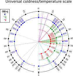
SI temperature/coldness conversion scale: Temperatures on the Kelvin scale are shown in blue (Celsius scale in green, Fahrenheit scale in red), coldness values in gigabyte per nanojoule are shown in black. Infinite temperature (coldness zero) is shown at the top of the diagram; positive values of coldness/temperature are on the right-hand side, negative values on the left-hand side.

Certain systems can achieve negative thermodynamic temperature; that is, their temperature can be expressed as a negative quantity on the Kelvin or Rankine scales. This should be distinguished from temperatures expressed as negative numbers on non-thermodynamic Celsius or Fahrenheit scales, which are nevertheless higher than absolute zero.

The absolute temperature (Kelvin) scale can be understood loosely as a measure of average kinetic energy. Usually, system temperatures are positive. However, in particular isolated systems, the temperature defined in terms of Boltzmann's entropy can become negative.

The possibility of negative temperatures was first predicted by Lars Onsager in 1949. ^[1] Onsager was investigating 2D vortices confined within a finite area, and realized that since their positions are not independent degrees of freedom from their momenta, the resulting phase space must also be bounded by the finite area. Bounded phase space is the essential property that allows for negative temperatures, and can occur in both classical and quantum systems. As shown by Onsager, a system with bounded phase space necessarily has a peak in the entropy as energy is increased. For energies exceeding the value where the peak occurs, the entropy decreases as energy increases, and high-energy states necessarily have negative Boltzmann temperature.

A system with a truly negative temperature on the Kelvin scale is hotter than any system with a positive temperature. If a negative-temperature system and a positive-temperature system come in contact, heat will flow from the negative- to the positive-temperature system. ^{[2] [3]} A standard example of such a system is population inversion in laser physics.

Temperature is loosely interpreted as the average kinetic energy of the system's particles. The existence of negative temperature, let alone negative temperature representing "hotter" systems than positive temperature, would seem paradoxical in this interpretation. The paradox is resolved by considering the more rigorous definition of thermodynamic temperature as the tradeoff between internal energy and entropy contained in the system, with "coldness", the reciprocal of temperature, being the more fundamental quantity. Systems with a positive temperature will increase in entropy as one adds energy to the system, while systems with a negative temperature will decrease in entropy as one adds energy to the system. ^[4]

Thermodynamic systems with unbounded phase space cannot achieve negative temperatures: adding heat always increases their entropy. The possibility of a decrease in entropy as energy increases requires the system to "saturate" in entropy. This is only possible if the number of high energy states is limited. For a system of ordinary (quantum or classical) particles such as atoms or dust, the number of high energy states is unlimited (particle momenta can in principle be increased indefinitely). Some systems, however (see the examples below), have a maximum amount of energy that they can hold, and as they approach that maximum energy their entropy actually begins to decrease. ^[5] The limited range of states accessible to a system with negative temperature means that negative temperature is associated with emergent ordering of the system at high energies. For example in Onsager's point-vortex analysis negative temperature is associated with the emergence of large-scale clusters of vortices. ^[1] This spontaneous ordering in equilibrium statistical mechanics goes against common physical intuition that increased energy leads to increased disorder.

Definition of temperature

The definition of thermodynamic temperature T is a function of the change in the system's entropy S under reversible heat transfer Q_rev:

${\displaystyle T={\frac {dQ_{\mathrm {rev} }}{dS}}.}$

Entropy being a state function, the integral of dS over any cyclical process is zero. For a system in which the entropy is purely a function of the system's energy E, the temperature can be defined as:

${\displaystyle T=\left({\frac {dS}{dE}}\right)^{-1}.}$

Equivalently, thermodynamic beta, or "coldness", is defined as

${\displaystyle \beta ={\frac {1}{kT}}={\frac {1}{k}}{\frac {dS}{dE}},}$

where k is the Boltzmann constant.

Note that in classical thermodynamics, S is defined in terms of temperature. This is reversed here, S is the statistical entropy, a function of the possible microstates of the system, and temperature conveys information on the distribution of energy levels among the possible microstates. For systems with many degrees of freedom, the statistical and thermodynamic definitions of entropy are generally consistent with each other.

Some theorists have proposed using an alternative definition of entropy as a way to resolve perceived inconsistencies between statistical and thermodynamic entropy for small systems and systems where the number of states decreases with energy, and the temperatures derived from these entropies are different. ^{[6] [7]} It has been argued that the new definition would create other inconsistencies; ^[8] its proponents have argued that this is only apparent. ^[7]

Heat and molecular energy distribution

When the temperature is negative, higher energy states are more likely to be occupied than low energy ones.

Negative temperatures can only exist in a system where there are a limited number of energy states (see below). As the temperature is increased on such a system, particles move into higher and higher energy states, and as the temperature increases, the number of particles in the lower energy states and in the higher energy states approaches equality. (This is a consequence of the definition of temperature in statistical mechanics for systems with limited states.) By injecting energy into these systems in the right fashion, it is possible to create a system in which there are more particles in the higher energy states than in the lower ones. The system can then be characterised as having a negative temperature.

A substance with a negative temperature is not colder than absolute zero, but rather it is hotter than infinite temperature. As Kittel and Kroemer (p. 462) put it,

The temperature scale from cold to hot runs:

:+0 K (−273.15 °C), …, +100 K (−173.15 °C), …, +300 K (+26.85 °C), …, +1000 K (+726.85 °C), …, +∞ K (+∞ °C), −∞ K (−∞ °C), …, −1000 K (−1273.15 °C), …, −300 K (−573.15 °C), …, −100 K (−373.15 °C), …, −0 K (−273.15 °C).

The corresponding inverse temperature scale, for the quantity β = 1/kT (where k is the Boltzmann constant), runs continuously from low energy to high as +∞, …, 0, …, −∞. Because it avoids the abrupt jump from +∞ to −∞, β is considered more natural than T. Although a system can have multiple negative temperature regions and thus have −∞ to +∞ discontinuities.

In many familiar physical systems, temperature is associated to the kinetic energy of atoms. Since there is no upper bound on the momentum of an atom, there is no upper bound to the number of energy states available when more energy is added, and therefore no way to get to a negative temperature. However, in statistical mechanics, temperature can correspond to other degrees of freedom than just kinetic energy (see below).

Temperature and disorder

The distribution of energy among the various translational, vibrational, rotational, electronic, and nuclear modes of a system determines the macroscopic temperature. In a "normal" system, thermal energy is constantly being exchanged between the various modes.

However, in some situations, it is possible to isolate one or more of the modes. In practice, the isolated modes still exchange energy with the other modes, but the time scale of this exchange is much slower than for the exchanges within the isolated mode. One example is the case of nuclear spins in a strong external magnetic field. In this case, energy flows fairly rapidly among the spin states of interacting atoms, but energy transfer between the nuclear spins and other modes is relatively slow. Since the energy flow is predominantly within the spin system, it makes sense to think of a spin temperature that is distinct from the temperature associated to other modes.

A definition of temperature can be based on the relationship:

${\displaystyle T={\frac {dq_{\mathrm {rev} }}{dS}}}$

The relationship suggests that a positive temperature corresponds to the condition where entropy, S, increases as thermal energy, q_rev, is added to the system. This is the "normal" condition in the macroscopic world, and is always the case for the translational, vibrational, rotational, and non-spin-related electronic and nuclear modes. The reason for this is that there are an infinite number of these types of modes, and adding more heat to the system increases the number of modes that are energetically accessible, and thus increases the entropy.

Examples

Noninteracting two-level particles

Entropy, thermodynamic beta, and temperature as a function of the energy for a system of N noninteracting two-level particles.

The simplest example, albeit a rather nonphysical one, is to consider a system of N particles, each of which can take an energy of either +ε or −ε but are otherwise noninteracting. This can be understood as a limit of the Ising model in which the interaction term becomes negligible. The total energy of the system is

${\displaystyle E=\varepsilon \sum _{i=1}^{N}\sigma _{i}=\varepsilon j}$

where σ_i is the sign of the ith particle and j is the number of particles with positive energy minus the number of particles with negative energy. From elementary combinatorics, the total number of microstates with this amount of energy is a binomial coefficient:

${\displaystyle \Omega _{E}={\binom {N}{\frac {N+j}{2}}}={\frac {N!}{\left({\frac {N+j}{2}}\right)!\left({\frac {N-j}{2}}\right)!}}.}$

By the fundamental assumption of statistical mechanics, the entropy of this microcanonical ensemble is

${\displaystyle S=k_{\text{B}}\ln \Omega _{E}}$

We can solve for thermodynamic beta (β = 1/k_BT) by considering it as a central difference without taking the continuum limit:

${\displaystyle {\begin{aligned}\beta &={\frac {1}{k_{\mathrm {B} }}}{\frac {\delta _{2\varepsilon }[S]}{2\varepsilon }}\\[3pt]&={\frac {1}{2\varepsilon }}\left(\ln \Omega _{E+\varepsilon }-\ln \Omega _{E-\varepsilon }\right)\\[3pt]&={\frac {1}{2\varepsilon }}\ln \left({\frac {\left({\frac {N+j-1}{2}}\right)!\left({\frac {N-j+1}{2}}\right)!}{\left({\frac {N+j+1}{2}}\right)!\left({\frac {N-j-1}{2}}\right)!}}\right)\\[3pt]&={\frac {1}{2\varepsilon }}\ln \left({\frac {N-j+1}{N+j+1}}\right).\end{aligned}}}$

hence the temperature

${\displaystyle T(E)={\frac {2\varepsilon }{k_{\text{B}}}}\left[\ln \left({\frac {(N+1)\varepsilon -E}{(N+1)\varepsilon +E}}\right)\right]^{-1}.}$

This entire proof assumes the microcanonical ensemble with energy fixed and temperature being the emergent property. In the canonical ensemble, the temperature is fixed and energy is the emergent property. This leads to (ε refers to microstates):

${\displaystyle {\begin{aligned}Z(T)&=\sum _{i=1}^{N}e^{-\varepsilon _{i}\beta }\\[6pt]E(T)&={\frac {1}{Z}}\sum _{i=1}^{N}\varepsilon _{i}e^{-\varepsilon _{i}\beta }\\[6pt]S(T)&=k_{\text{B}}\ln(Z)+{\frac {E}{T}}\end{aligned}}}$

Following the previous example, we choose a state with two levels and two particles. This leads to microstates ε₁ = 0, ε₂ = 1, ε₃ = 1, and ε₄ = 2.

${\displaystyle {\begin{aligned}Z(T)&=e^{-0\beta }+2e^{-1\beta }+e^{-2\beta }\\[3pt]&=1+2e^{-\beta }+e^{-2\beta }\\[6pt]E(T)&={\frac {0e^{-0\beta }+2\times 1e^{-1\beta }+2e^{-2\beta }}{Z}}\\[3pt]&={\frac {2e^{-\beta }+2e^{-2\beta }}{Z}}\\[3pt]&={\frac {2e^{-\beta }+2e^{-2\beta }}{1+2e^{-\beta }+e^{-2\beta }}}\\[6pt]S(T)&=k_{\text{B}}\ln \left(1+2e^{-\beta }+e^{-2\beta }\right)+{\frac {2e^{-\beta }+2e^{-2\beta }}{\left(1+2e^{-\beta }+e^{-2\beta }\right)T}}\end{aligned}}}$

The resulting values for S, E, and Z all increase with T and never need to enter a negative temperature regime.

Nuclear spins

The previous example is approximately realized by a system of nuclear spins in an external magnetic field. ^{[9] [10]} This allows the experiment to be run as a variation of nuclear magnetic resonance spectroscopy. In the case of electronic and nuclear spin systems, there are only a finite number of modes available, often just two, corresponding to spin up and spin down. In the absence of a magnetic field, these spin states are degenerate, meaning that they correspond to the same energy. When an external magnetic field is applied, the energy levels are split, since those spin states that are aligned with the magnetic field will have a different energy from those that are anti-parallel to it.

In the absence of a magnetic field, such a two-spin system would have maximum entropy when half the atoms are in the spin-up state and half are in the spin-down state, and so one would expect to find the system with close to an equal distribution of spins. Upon application of a magnetic field, some of the atoms will tend to align so as to minimize the energy of the system, thus slightly more atoms should be in the lower-energy state (for the purposes of this example we will assume the spin-down state is the lower-energy state). It is possible to add energy to the spin system using radio frequency techniques. ^[11] This causes atoms to flip from spin-down to spin-up.

Since we started with over half the atoms in the spin-down state, this initially drives the system towards a 50/50 mixture, so the entropy is increasing, corresponding to a positive temperature. However, at some point, more than half of the spins are in the spin-up position. ^[12] In this case, adding additional energy reduces the entropy, since it moves the system further from a 50/50 mixture. This reduction in entropy with the addition of energy corresponds to a negative temperature. ^[13] In NMR spectroscopy, this corresponds to pulses with a pulse width of over 180° (for a given spin). While relaxation is fast in solids, it can take several seconds in solutions and even longer in gases and in ultracold systems; several hours were reported for silver and rhodium at picokelvin temperatures. ^[13] It is still important to understand that the temperature is negative only with respect to nuclear spins. Other degrees of freedom, such as molecular vibrational, electronic and electron spin levels are at a positive temperature, so the object still has positive sensible heat. Relaxation actually happens by exchange of energy between the nuclear spin states and other states (e.g. through the nuclear Overhauser effect with other spins).

Lasers

This phenomenon can also be observed in many lasing systems, wherein a large fraction of the system's atoms (for chemical and gas lasers) or electrons (in semiconductor lasers) are in excited states. This is referred to as a population inversion.

The Hamiltonian for a single mode of a luminescent radiation field at frequency ν is

${\displaystyle H=(h\nu -\mu )a^{\dagger }a.}$

The density operator in the grand canonical ensemble is

${\displaystyle \rho ={\frac {e^{-\beta H}}{\operatorname {Tr} \left(e^{-\beta H}\right)}}.}$

For the system to have a ground state, the trace to converge, and the density operator to be generally meaningful, βH must be positive semidefinite. So if hν < μ, and H is negative semidefinite, then β must itself be negative, implying a negative temperature. ^[14]

Motional degrees of freedom

Negative temperatures have also been achieved in motional degrees of freedom. Using an optical lattice, upper bounds were placed on the kinetic energy, interaction energy and potential energy of cold potassium-39 atoms. This was done by tuning the interactions of the atoms from repulsive to attractive using a Feshbach resonance and changing the overall harmonic potential from trapping to anti-trapping, thus transforming the Bose-Hubbard Hamiltonian from Ĥ → −Ĥ. Performing this transformation adiabatically while keeping the atoms in the Mott insulator regime, it is possible to go from a low entropy positive temperature state to a low entropy negative temperature state. In the negative temperature state, the atoms macroscopically occupy the maximum momentum state of the lattice. The negative temperature ensembles equilibrated and showed long lifetimes in an anti-trapping harmonic potential. ^[15]

Two-dimensional vortex motion

The two-dimensional systems of vortices confined to a finite area can form thermal equilibrium states at negative temperature, ^{[16] [17]} and indeed negative temperature states were first predicted by Onsager in his analysis of classical point vortices. ^[18] Onsager's prediction was confirmed experimentally for a system of quantum vortices in a Bose-Einstein condensate in 2019. ^{[19] [20]}

See also

• Negative resistance

References

1. Onsager, L. (1949). "Statistical Hydrodynamics". Il Nuovo Cimento. 6 (2): 279–287. Bibcode:1949NCim....6S.279O. doi:10.1007/BF02780991. ISSN   1827-6121. S2CID   186224016.
2. Ramsey, Norman (1956-07-01). "Thermodynamics and Statistical Mechanics at Negative Absolute Temperatures". Physical Review. 103 (1): 20–28. Bibcode:1956PhRv..103...20R. doi:10.1103/PhysRev.103.20.
3. Tremblay, André-Marie (1975-11-18). "Comment on: Negative Kelvin temperatures: some anomalies and a speculation" (PDF). American Journal of Physics. 44 (10): 994–995. Bibcode:1976AmJPh..44..994T. doi:10.1119/1.10248.
4. Atkins, Peter W. (2010-03-25). The Laws of Thermodynamics: A Very Short Introduction. Oxford University Press. pp. 10–14. ISBN   978-0-19-957219-9. OCLC   467748903.
5. Atkins, Peter W. (2010-03-25). The Laws of Thermodynamics: A Very Short Introduction. Oxford University Press. pp. 89–95. ISBN   978-0-19-957219-9. OCLC   467748903.
6. Dunkel, Jorn; Hilbert, Stefan (2013). "Consistent thermostatistics forbids negative absolute temperatures". Nature Physics. 10 (1): 67. arXiv: 1304.2066 . Bibcode:2014NatPh..10...67D. doi:10.1038/nphys2815. S2CID   16757018.
7. Hanggi, Peter; Hilbert, Stefan; Dunkel, Jorn (2016). "Meaning of temperature in different thermostatistical ensembles". Philosophical Transactions of the Royal Society A: Mathematical, Physical and Engineering Sciences. 374 (2064): 20150039. arXiv: 1507.05713 . Bibcode:2016RSPTA.37450039H. doi:10.1098/rsta.2015.0039. PMID   26903095. S2CID   39161351.
8. Frenkel, Daan; Warren, Patrick B. (2015-02-01). "Gibbs, Boltzmann, and negative temperatures". American Journal of Physics. 83 (2): 163–170. arXiv: 1403.4299 . Bibcode:2015AmJPh..83..163F. doi:10.1119/1.4895828. ISSN   0002-9505. S2CID   119179342.
9. Purcell, E. M.; Pound, R. V. (1951-01-15). "A Nuclear Spin System at Negative Temperature". Physical Review. 81 (2): 279–280. Bibcode:1951PhRv...81..279P. doi:10.1103/PhysRev.81.279.
10. Varga, Peter (1998). "Minimax games, spin glasses, and the polynomial-time hierarchy of complexity classes". Physical Review E. 57 (6): 6487–6492. arXiv: cond-mat/9604030 . Bibcode:1998PhRvE..57.6487V. CiteSeerX   10.1.1.306.470 . doi:10.1103/PhysRevE.57.6487. S2CID   10964509.
11. Ramsey, Norman F. (1998). Spectroscopy with coherent radiation: selected papers of Norman F. Ramsey with commentary. World Scientific series in 20th century physics, v. 21. Singapore; River Edge, N.J.: World Scientific. p. 417. ISBN   9789810232504. OCLC   38753008.
12. Levitt, Malcolm H. (2008). Spin Dynamics: Basics of Nuclear Magnetic Resonance. West Sussex, England: John Wiley & Sons Ltd. p. 273. ISBN   978-0-470-51117-6.
13. "Positive and negative picokelvin temperatures".
14. Hsu, W.; Barakat, R. (1992). "Statistics and thermodynamics of luminescent radiation". Physical Review B . 46 (11): 6760–6767. Bibcode:1992PhRvB..46.6760H. doi:10.1103/PhysRevB.46.6760. PMID   10002377.
15. Braun, S.; Ronzheimer, J. P.; Schreiber, M.; Hodgman, S. S.; Rom, T.; Bloch, I.; Schneider, U. (2013). "Negative Absolute Temperature for Motional Degrees of Freedom". Science. 339 (6115): 52–55. arXiv: 1211.0545 . Bibcode:2013Sci...339...52B. doi:10.1126/science.1227831. PMID   23288533. S2CID   8207974.
16. Montgomery, D. C. (1972). "Two-dimensional vortex motion and "negative temperatures"". Physics Letters A . 39 (1): 7–8. Bibcode:1972PhLA...39....7M. doi:10.1016/0375-9601(72)90302-7.
17. Edwards, S. F.; Taylor, J. B. (1974). "Negative Temperature States of Two-Dimensional Plasmas and Vortex Fluids". Proceedings of the Royal Society of London A . 336 (1606): 257–271. Bibcode:1974RSPSA.336..257E. doi:10.1098/rspa.1974.0018. JSTOR   78450. S2CID   120771020.
18. Onsager, L. (1949-03-01). "Statistical hydrodynamics". Il Nuovo Cimento (1943-1954). 6 (2): 279–287. Bibcode:1949NCim....6S.279O. doi:10.1007/BF02780991. ISSN   1827-6121. S2CID   186224016 . Retrieved 2019-11-17.
19. Gauthier, G.; Reeves, M. T.; Yu, X.; Bradley, A. S.; Baker, M. A.; Bell, T. A.; Rubinsztein-Dunlop, H.; Davis, M. J.; Neely, T. W. (2019). "Giant vortex clusters in a two-dimensional quantum fluid". Science. 364 (6447): 1264–1267. arXiv: 1801.06951 . Bibcode:2019Sci...364.1264G. doi:10.1126/science.aat5718. PMID   31249054. S2CID   195750381.
20. Johnstone, S. P.; Groszek, A. J.; Starkey, P. T.; Billinton, C. J.; Simula, T. P.; Helmerson, K. (2019). "Evolution of large-scale flow from turbulence in a two-dimensional superfluid". Science. 365 (6447): 1267–1271. arXiv: 1801.06952 . Bibcode:2019Sci...364.1267J. doi:10.1126/science.aat5793. PMID   31249055. S2CID   4948239.

Further reading

• Kittel, C.; Kroemer, H. (1980). Thermal Physics (2nd ed.). W. H. Freeman. ISBN   978-0-7167-1088-2.
• Castle, J.; Emmerich, W.; Heikes, R.; Miller, R.; Rayne, J. (1965). Science by Degrees: Temperature from Zero to Zero. Walker and Company. LCCN   64023985.
• Braun, S.; Ronzheimer, J. P.; Schreiber, M.; Hodgman, S. S.; Rom, T.; Bloch, I.; Schneider, U. (2013). "Negative Absolute Temperature for Motional Degrees of Freedom". Science. 339 (6115): 52–5. arXiv: 1211.0545 . Bibcode:2013Sci...339...52B. doi:10.1126/science.1227831. PMID   23288533. S2CID   8207974.
• Parihar, V.; Widom, A.; Srivastava, Y. (2006). "Thermal Time Scales in a Color Glass Condensate". Physical Review C. 73 (17901): 017901. arXiv: hep-ph/0505199 . Bibcode:2006PhRvC..73a7901P. doi:10.1103/PhysRevC.73.017901. S2CID   119090586.
• Mosk, A. (2005). "Atomic Gases at Negative Kinetic Temperature". Physical Review Letters. 95 (4): 040403. arXiv: cond-mat/0501344 . Bibcode:2005PhRvL..95d0403M. doi:10.1103/PhysRevLett.95.040403. PMID   16090784. S2CID   1156732.
• Schmidt, Harry; Mahler, Günter (2005). "Control of Local Relaxation Behavior in Closed Bipartite Quantum Systems". Physical Review E. 72 (7): 016117. arXiv: quant-ph/0502181 . Bibcode:2005PhRvE..72a6117S. doi:10.1103/PhysRevE.72.016117. PMID   16090046. S2CID   17987338.
• Shen, Jian-Qi (2003). "Anti-shielding Effect and Negative Temperature in Instantaneously Reversed Electric Fields and Left-Handed Media". Physica Scripta. 68 (1): 87–97. arXiv: cond-mat/0302351 . Bibcode:2003PhyS...68...87S. doi:10.1238/Physica.Regular.068a00087. S2CID   118894011.
• Ketterle, Wolfgang (22 Sep 2010). Towards Quantum Magnetism with Ultracold Atoms (movie). The Zurich Physics Colloquium. ETH Zurich, ITS-MMS; Switzerland. Retrieved 1 Jan 2016. Negative temperature, at about 48min. 53sec.
• Carr, Lincoln D. (2013-01-04). "Negative Temperatures?". Science. 339 (6115): 42–43. Bibcode:2013Sci...339...42C. doi:10.1126/science.1232558. PMID   23288530. S2CID   124095369.

External links

• Moriarty, Philip. "−K: Negative Temperatures". Sixty Symbols. Brady Haran for the University of Nottingham.