Regular complex polygon

Three views of regular complex polygon₄{4}₂,

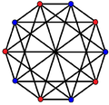
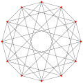
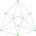
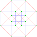
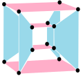
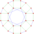
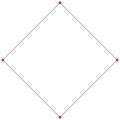
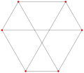
This complex polygon has 8 edges (complex lines), labeled as a..h, and 16 vertices. Four vertices lie in each edge and two edges intersect at each vertex. In the left image, the outlined squares are not elements of the polytope but are included merely to help identify vertices lying in the same complex line. The octagonal perimeter of the left image is not an element of the polytope, but it is a petrie polygon. [1] In the middle image, each edge is represented as a real line and the four vertices in each line can be more clearly seen.

A perspective sketch representing the 16 vertex points as large black dots and the 8 4-edges as bounded squares within each edge. The green path represents the octagonal perimeter of the left hand image.

Complex 1-polytopes represented in the Argand plane as regular polygons for p = 2, 3, 4, 5, and 6, with black vertices. The centroid of the p vertices is shown seen in red. The sides of the polygons represent one application of the symmetry generator, mapping each vertex to the next counterclockwise copy. These polygonal sides are not edge elements of the polytope, as a complex 1-polytope can have no edges (it often is a complex edge) and only contains vertex elements.

In geometry, a regular complex polygon is a generalization of a regular polygon in real space to an analogous structure in a complex Hilbert space, where each real dimension is accompanied by an imaginary one. A regular polygon exists in 2 real dimensions, ${\displaystyle \mathbb {R} ^{2}}$, while a complex polygon exists in two complex dimensions, ${\displaystyle \mathbb {C} ^{2}}$, which can be given real representations in 4 dimensions, ${\displaystyle \mathbb {R} ^{4}}$, which then must be projected down to 2 or 3 real dimensions to be visualized. A complex polygon is generalized as a complex polytope in ${\displaystyle \mathbb {C} ^{n}}$.

A complex polygon may be understood as a collection of complex points, lines, planes, and so on, where every point is the junction of multiple lines, every line of multiple planes, and so on.

The regular complex polygons have been completely characterized, and can be described using a symbolic notation developed by Coxeter.

A regular complex polygon with all 2-edges can be represented by a graph, while forms with k-edges can only be related by hypergraphs. A k-edge can be seen as a set of vertices, with no order implied. They may be drawn with pairwise 2-edges, but this is not structurally accurate.

Regular complex polygons

While 1-polytopes can have unlimited p, finite regular complex polygons, excluding the double prism polygons _p{4}₂, are limited to 5-edge (pentagonal edges) elements, and infinite regular apeirogons also include 6-edge (hexagonal edges) elements.

Notations

Shephard's modified Schläfli notation

Shephard originally devised a modified form of Schläfli's notation for regular polytopes. For a polygon bounded by p₁-edges, with a p₂-set as vertex figure and overall symmetry group of order g, we denote the polygon as p₁(g)p₂.

The number of vertices V is then g/p₂ and the number of edges E is g/p₁.

The complex polygon illustrated above has eight square edges (p₁=4) and sixteen vertices (p₂=2). From this we can work out that g = 32, giving the modified Schläfli symbol 4(32)2.

Coxeter's revised modified Schläfli notation

A more modern notation _p1{q}_p2 is due to Coxeter, ^[2] and is based on group theory. As a symmetry group, its symbol is _p1[q]_p2.

The symmetry group _p1[q]_p2 is represented by 2 generators R₁, R₂, where: R₁^p₁ = R₂^p₂ = I. If q is even, (R₂R₁)^q/2 = (R₁R₂)^q/2. If q is odd, (R₂R₁)^(q−1)/2R₂ = (R₁R₂)^(q−1)/2R₁. When q is odd, p₁=p₂.

For ₄[4]₂ has R₁⁴ = R₂² = I, (R₂R₁)² = (R₁R₂)².

For ₃[5]₃ has R₁³ = R₂³ = I, (R₂R₁)²R₂ = (R₁R₂)²R₁.

Coxeter–Dynkin diagrams

Coxeter also generalised the use of Coxeter–Dynkin diagrams to complex polytopes, for example the complex polygon _p{q}_r is represented by and the equivalent symmetry group, _p[q]_r, is a ringless diagram . The nodes p and r represent mirrors producing p and r images in the plane. Unlabeled nodes in a diagram have implicit 2 labels. For example, a real regular polygon is ₂{q}₂ or {q} or .

One limitation, nodes connected by odd branch orders must have identical node orders. If they do not, the group will create "starry" polygons, with overlapping element. So and are ordinary, while is starry.

12 Irreducible Shephard groups

12 irreducible Shephard groups with their subgroup index relations. [3]	Subgroups from <5,3,2>30, <4,3,2>12 and <3,3,2>6
Subgroups relate by removing one reflection: p[2q]2 --> p[q]p, index 2 and p[4]q --> p[q]p, index q.

_p[4]₂ subgroups: p=2,3,4...
_p[4]₂ --> [p], index p
_p[4]₂ --> _p[]×_p[], index 2

Coxeter enumerated this list of regular complex polygons in ${\displaystyle \mathbb {C} ^{2}}$. A regular complex polygon, _p{q}_r or , has p-edges, and r-gonal vertex figures. _p{q}_r is a finite polytope if (p + r)q > pr(q − 2).

Its symmetry is written as _p[q]_r, called a Shephard group , analogous to a Coxeter group, while also allowing unitary reflections.

For nonstarry groups, the order of the group _p[q]_r can be computed as ${\displaystyle g=8/q\cdot (1/p+2/q+1/r-1)^{-2}}$. ^[4]

The Coxeter number for _p[q]_r is ${\displaystyle h=2/(1/p+2/q+1/r-1)}$, so the group order can also be computed as ${\displaystyle g=2h^{2}/q}$. A regular complex polygon can be drawn in orthogonal projection with h-gonal symmetry.

The rank 2 solutions that generate complex polygons are:

Group	G3 = G(q,1,1)	G2 = G(p,1,2)	G4	G6	G5	G8	G14	G9	G10	G20	G16	G21	G17	G18
	2[q]2, q = 3,4...	p[4]2, p = 2,3...	3[3]3	3[6]2	3[4]3	4[3]4	3[8]2	4[6]2	4[4]3	3[5]3	5[3]5	3[10]2	5[6]2	5[4]3
Order	2q	2p2	24	48	72	96	144	192	288	360	600	720	1200	1800
h	q	2p	6	12			24			30		60

Excluded solutions with odd q and unequal p and r are: ₆[3]₂, ₆[3]₃, ₉[3]₃, ₁₂[3]₃, ..., ₅[5]₂, ₆[5]₂, ₈[5]₂, ₉[5]₂, ₄[7]₂, ₉[5]₂, ₃[9]₂, and ₃[11]₂.

Other whole q with unequal p and r, create starry groups with overlapping fundamental domains: , , , , , and .

The dual polygon of _p{q}_r is _r{q}_p. A polygon of the form _p{q}_p is self-dual. Groups of the form _p[2q]₂ have a half symmetry _p[q]_p, so a regular polygon is the same as quasiregular . As well, regular polygon with the same node orders, , have an alternated construction , allowing adjacent edges to be two different colors. ^[5]

The group order, g, is used to compute the total number of vertices and edges. It will have g/r vertices, and g/p edges. When p=r, the number of vertices and edges are equal. This condition is required when q is odd.

Matrix generators

The group p[q]r, , can be represented by two matrices: ^[6]

Name	R1	R2
Order	p	r
Matrix	${\displaystyle \left[{\begin{smallmatrix}e^{2\pi i/p}&0\\(e^{2\pi i/p}-1)k&1\\\end{smallmatrix}}\right]}$	${\displaystyle \left[{\begin{smallmatrix}1&(e^{2\pi i/r}-1)k\\0&e^{2\pi i/r}\end{smallmatrix}}\right]}$

With

${\displaystyle k={\sqrt {\frac {\cos({\frac {\pi }{p}}-{\frac {\pi }{r}})+\cos({\frac {2\pi }{q}})}{2\sin {\frac {\pi }{p}}\sin {\frac {\pi }{r}}}}}}$

Examples

Name R1 R2 Order p q Matrix ${\displaystyle \left[{\begin{smallmatrix}e^{2\pi i/p}&0\\0&1\\\end{smallmatrix}}\right]}$ ${\displaystyle \left[{\begin{smallmatrix}1&0\\0&e^{2\pi i/q}\\\end{smallmatrix}}\right]}$	Name R1 R2 Order p 2 Matrix ${\displaystyle \left[{\begin{smallmatrix}e^{2\pi i/p}&0\\0&1\\\end{smallmatrix}}\right]}$ ${\displaystyle \left[{\begin{smallmatrix}0&1\\1&0\\\end{smallmatrix}}\right]}$	Name R1 R2 Order 3 3 Matrix ${\displaystyle \left[{\begin{smallmatrix}{\frac {-1+{\sqrt {3}}i}{2}}&0\\{\frac {-3+{\sqrt {3}}i}{2}}&1\\\end{smallmatrix}}\right]}$ ${\displaystyle \left[{\begin{smallmatrix}1&{\frac {-3+{\sqrt {3}}i}{2}}\\0&{\frac {-1+{\sqrt {3}}i}{2}}\\\end{smallmatrix}}\right]}$
Name R1 R2 Order 4 4 Matrix ${\displaystyle \left[{\begin{smallmatrix}i&0\\0&1\\\end{smallmatrix}}\right]}$ ${\displaystyle \left[{\begin{smallmatrix}1&0\\0&i\\\end{smallmatrix}}\right]}$	Name R1 R2 Order 4 2 Matrix ${\displaystyle \left[{\begin{smallmatrix}i&0\\0&1\\\end{smallmatrix}}\right]}$ ${\displaystyle \left[{\begin{smallmatrix}0&1\\1&0\\\end{smallmatrix}}\right]}$	Name R1 R2 Order 3 2 Matrix ${\displaystyle \left[{\begin{smallmatrix}{\frac {-1+{\sqrt {3}}i}{2}}&0\\{\frac {-3+{\sqrt {3}}i}{2}}&1\\\end{smallmatrix}}\right]}$ ${\displaystyle \left[{\begin{smallmatrix}1&-2\\0&-1\\\end{smallmatrix}}\right]}$

Enumeration of regular complex polygons

Coxeter enumerated the complex polygons in Table III of Regular Complex Polytopes. ^[7]

Group	Order	Coxeter number	Polygon		Vertices	Edges		Notes
G(q,q,2) 2[q]2 = [q] q = 2,3,4,...	2q	q	2{q}2		q	q	{}	Real regular polygons Same as Same as if q even

Group	Order	Coxeter number	Polygon			Vertices	Edges		Notes
G(p,1,2) p[4]2 p=2,3,4,...	2p2	2p	p(2p2)2	p{4}2		p2	2p	p{}	same as p{}×p{} or ${\displaystyle \mathbb {R} ^{4}}$ representation as p-p duoprism
			2(2p2)p	2{4}p		2p	p2	{}	${\displaystyle \mathbb {R} ^{4}}$ representation as p-p duopyramid
G(2,1,2) 2[4]2 = [4]	8	4		2{4}2 = {4}		4	4	{}	same as {}×{} or Real square
G(3,1,2) 3[4]2	18	6	6(18)2	3{4}2		9	6	3{}	same as 3{}×3{} or ${\displaystyle \mathbb {R} ^{4}}$ representation as 3-3 duoprism
			2(18)3	2{4}3		6	9	{}	${\displaystyle \mathbb {R} ^{4}}$ representation as 3-3 duopyramid
G(4,1,2) 4[4]2	32	8	8(32)2	4{4}2		16	8	4{}	same as 4{}×4{} or ${\displaystyle \mathbb {R} ^{4}}$ representation as 4-4 duoprism or {4,3,3}
			2(32)4	2{4}4		8	16	{}	${\displaystyle \mathbb {R} ^{4}}$ representation as 4-4 duopyramid or {3,3,4}
G(5,1,2) 5[4]2	50	25	5(50)2	5{4}2		25	10	5{}	same as 5{}×5{} or ${\displaystyle \mathbb {R} ^{4}}$ representation as 5-5 duoprism
			2(50)5	2{4}5		10	25	{}	${\displaystyle \mathbb {R} ^{4}}$ representation as 5-5 duopyramid
G(6,1,2) 6[4]2	72	36	6(72)2	6{4}2		36	12	6{}	same as 6{}×6{} or ${\displaystyle \mathbb {R} ^{4}}$ representation as 6-6 duoprism
			2(72)6	2{4}6		12	36	{}	${\displaystyle \mathbb {R} ^{4}}$ representation as 6-6 duopyramid
G4=G(1,1,2) 3[3]3 <2,3,3>	24	6	3(24)3	3{3}3		8	8	3{}	Möbius–Kantor configuration self-dual, same as ${\displaystyle \mathbb {R} ^{4}}$ representation as {3,3,4}
G6 3[6]2	48	12	3(48)2	3{6}2		24	16	3{}	same as
				3{3}2					starry polygon
			2(48)3	2{6}3		16	24	{}
				2{3}3					starry polygon
G5 3[4]3	72	12	3(72)3	3{4}3		24	24	3{}	self-dual, same as ${\displaystyle \mathbb {R} ^{4}}$ representation as {3,4,3}
G8 4[3]4	96	12	4(96)4	4{3}4		24	24	4{}	self-dual, same as ${\displaystyle \mathbb {R} ^{4}}$ representation as {3,4,3}
G14 3[8]2	144	24	3(144)2	3{8}2		72	48	3{}	same as
				3{8/3}2					starry polygon, same as
			2(144)3	2{8}3		48	72	{}
				2{8/3}3					starry polygon
G9 4[6]2	192	24	4(192)2	4{6}2		96	48	4{}	same as
			2(192)4	2{6}4		48	96	{}
				4{3}2		96	48	{}	starry polygon
				2{3}4		48	96	{}	starry polygon
G10 4[4]3	288	24	4(288)3	4{4}3		96	72	4{}
		12		4{8/3}3					starry polygon
		24	3(288)4	3{4}4		72	96	3{}
		12		3{8/3}4					starry polygon
G20 3[5]3	360	30	3(360)3	3{5}3		120	120	3{}	self-dual, same as ${\displaystyle \mathbb {R} ^{4}}$ representation as {3,3,5}
				3{5/2}3					self-dual, starry polygon
G16 5[3]5	600	30	5(600)5	5{3}5		120	120	5{}	self-dual, same as ${\displaystyle \mathbb {R} ^{4}}$ representation as {3,3,5}
		10		5{5/2}5					self-dual, starry polygon
G21 3[10]2	720	60	3(720)2	3{10}2		360	240	3{}	same as
				3{5}2					starry polygon
				3{10/3}2					starry polygon, same as
				3{5/2}2					starry polygon
			2(720)3	2{10}3		240	360	{}
				2{5}3					starry polygon
				2{10/3}3					starry polygon
				2{5/2}3					starry polygon
G17 5[6]2	1200	60	5(1200)2	5{6}2		600	240	5{}	same as
		20		5{5}2					starry polygon
		20		5{10/3}2					starry polygon
		60		5{3}2					starry polygon
		60	2(1200)5	2{6}5		240	600	{}
		20		2{5}5					starry polygon
		20		2{10/3}5					starry polygon
		60		2{3}5					starry polygon
G18 5[4]3	1800	60	5(1800)3	5{4}3		600	360	5{}
		15		5{10/3}3					starry polygon
		30		5{3}3					starry polygon
		30		5{5/2}3					starry polygon
		60	3(1800)5	3{4}5		360	600	3{}
		15		3{10/3}5					starry polygon
		30		3{3}5					starry polygon
		30		3{5/2}5					starry polygon

Visualizations of regular complex polygons

2D graphs

Polygons of the form _p{2r}_q can be visualized by q color sets of p-edge. Each p-edge is seen as a regular polygon, while there are no faces.

Complex polygons ₂{r}_q

Polygons of the form ₂{4}_q are called generalized orthoplexes. They share vertices with the 4D q-q duopyramids, vertices connected by 2-edges.

• 
  ₂{4}₂, , with 4 vertices, and 4 edges
• 
  ₂{4}₃, , with 6 vertices, and 9 edges ^[8]
• 
  ₂{4}₄, , with 8 vertices, and 16 edges
• 
  ₂{4}₅, , with 10 vertices, and 25 edges
• 
  ₂{4}₆, , with 12 vertices, and 36 edges
• 
  ₂{4}₇, , with 14 vertices, and 49 edges
• 
  ₂{4}₈, , with 16 vertices, and 64 edges
• 
  ₂{4}₉, , with 18 vertices, and 81 edges
• 
  ₂{4}₁₀, , with 20 vertices, and 100 edges

Complex polygons _p{4}₂

Polygons of the form _p{4}₂ are called generalized hypercubes (squares for polygons). They share vertices with the 4D p-p duoprisms, vertices connected by p-edges. Vertices are drawn in green, and p-edges are drawn in alternate colors, red and blue. The perspective is distorted slightly for odd dimensions to move overlapping vertices from the center.

• 
  ₂{4}₂, or , with 4 vertices, and 4 2-edges
• 
  ₃{4}₂, or , with 9 vertices, and 6 (triangular) 3-edges ^[9]
• 
  ₄{4}₂, or , with 16 vertices, and 8 (square) 4-edges
• 
  ₅{4}₂, or , with 25 vertices, and 10 (pentagonal) 5-edges
• 
  ₆{4}₂, or , with 36 vertices, and 12 (hexagonal) 6-edges
• 
  ₇{4}₂, or , with 49 vertices, and 14 (heptagonal)7-edges
• 
  ₈{4}₂, or , with 64 vertices, and 16 (octagonal) 8-edges
• 
  ₉{4}₂, or , with 81 vertices, and 18 (enneagonal) 9-edges
• 
  ₁₀{4}₂, or , with 100 vertices, and 20 (decagonal) 10-edges

Complex polygons _p{r}₂

• 
  ₃{6}₂, or , with 24 vertices in black, and 16 3-edges colored in 2 sets of 3-edges in red and blue ^[10]
• 
  ₃{8}₂, or , with 72 vertices in black, and 48 3-edges colored in 2 sets of 3-edges in red and blue ^[11]

Complex polygons, _p{r}_p

Polygons of the form _p{r}_p have equal number of vertices and edges. They are also self-dual.

• 
  ₃{3}₃, or , with 8 vertices in black, and 8 3-edges colored in 2 sets of 3-edges in red and blue ^[12]
• 
  ₃{4}₃, or , with 24 vertices and 24 3-edges shown in 3 sets of colors, one set filled ^[13]
• 
  ₄{3}₄, or , with 24 vertices and 24 4-edges shown in 4 sets of colors ^[14]
• 
  ₃{5}₃, or , with 120 vertices and 120 3-edges ^[15]
• 
  ₅{3}₅, or , with 120 vertices and 120 5-edges ^[16]

3D perspective

3D perspective projections of complex polygons _p{4}₂ can show the point-edge structure of a complex polygon, while scale is not preserved.

The duals ₂{4}_p: are seen by adding vertices inside the edges, and adding edges in place of vertices.

• 
  ₂{4}₃, with 6 vertices, 9 edges in 3 sets
• 
  ₃{4}₂, with 9 vertices, 6 3-edges in 2 sets of colors as
• 
  ₄{4}₂, with 16 vertices, 8 4-edges in 2 sets of colors and filled square 4-edges as
• 
  ₅{4}₂, with 25 vertices, 10 5-edges in 2 sets of colors as

Quasiregular polygons

A quasiregular polygon is a truncation of a regular polygon. A quasiregular polygon contains alternate edges of the regular polygons and . The quasiregular polygon has p vertices on the p-edges of the regular form.

Example quasiregular polygons

p[q]r	2[4]2	3[4]2	4[4]2	5[4]2	6[4]2	7[4]2	8[4]2	3[3]3	3[4]3
Regular	4 2-edges	9 3-edges	16 4-edges	25 5-edges	36 6-edges	49 7-edges	64 8-edges
Quasiregular	= 4+4 2-edges	6 2-edges 9 3-edges	8 2-edges 16 4-edges	10 2-edges 25 5-edges	12 2-edges 36 6-edges	14 2-edges 49 7-edges	16 2-edges 64 8-edges	=	=
Regular	4 2-edges	6 2-edges	8 2-edges	10 2-edges	12 2-edges	14 2-edges	16 2-edges

Notes

1. Coxeter, Regular Complex Polytopes, 11.3 Petrie Polygon, a simple h-gon formed by the orbit of the flag (O₀,O₀O₁) for the product of the two generating reflections of any nonstarry regular complex polygon, p₁{q}p₂.
2. Coxeter, Regular Complex Polytopes, p. xiv
3. Coxeter, Complex Regular Polytopes, p. 177, Table III
4. Lehrer & Taylor 2009, p. 87
5. Coxeter, Regular Complex Polytopes, Table IV. The regular polygons. pp. 178–179
6. Complex Polytopes, 8.9 The Two-Dimensional Case, p. 88
7. Regular Complex Polytopes, Coxeter, pp. 177–179
8. Coxeter, Regular Complex Polytopes, p. 108
9. Coxeter, Regular Complex Polytopes, p. 108
10. Coxeter, Regular Complex Polytopes, p. 109
11. Coxeter, Regular Complex Polytopes, p. 111
12. Coxeter, Regular Complex Polytopes, p. 30 diagram and p. 47 indices for 8 3-edges
13. Coxeter, Regular Complex Polytopes, p. 110
14. Coxeter, Regular Complex Polytopes, p. 110
15. Coxeter, Regular Complex Polytopes, p. 48
16. Coxeter, Regular Complex Polytopes, p. 49

References

• Coxeter, H.S.M. and Moser, W. O. J.; Generators and Relations for Discrete Groups (1965), esp pp 67–80.
• Coxeter, H.S.M. (1991), Regular Complex Polytopes, Cambridge University Press, ISBN   0-521-39490-2
• Coxeter, H.S.M. and Shephard, G.C.; Portraits of a family of complex polytopes, Leonardo Vol 25, No 3/4, (1992), pp 239–244,
• Shephard, G.C.; Regular complex polytopes, Proc. London math. Soc. Series 3, Vol 2, (1952), pp 82–97.
• G. C. Shephard, J. A. Todd, Finite unitary reflection groups, Canadian Journal of Mathematics. 6(1954), 274–304 ^[ permanent dead link ]
• Gustav I. Lehrer and Donald E. Taylor, Unitary Reflection Groups, Cambridge University Press 2009