
In celestial mechanics, an orbit is the curved trajectory of an object such as the trajectory of a planet around a star, or of a natural satellite around a planet, or of an artificial satellite around an object or position in space such as a planet, moon, asteroid, or Lagrange point. Normally, orbit refers to a regularly repeating trajectory, although it may also refer to a non-repeating trajectory. To a close approximation, planets and satellites follow elliptic orbits, with the center of mass being orbited at a focal point of the ellipse, as described by Kepler's laws of planetary motion.

A gyrocompass is a type of non-magnetic compass which is based on a fast-spinning disc and the rotation of the Earth to find geographical direction automatically. A gyrocompass makes use of one of the seven fundamental ways to determine the heading of a vehicle. A gyroscope is an essential component of a gyrocompass, but they are different devices; a gyrocompass is built to use the effect of gyroscopic precession, which is a distinctive aspect of the general gyroscopic effect. Gyrocompasses, such as the fibre optic gyrocompass are widely used to provide a heading for navigation on ships. This is because they have two significant advantages over magnetic compasses:

In physics, angular velocity, also known as angular frequency vector, is a pseudovector representation of how the angular position or orientation of an object changes with time, i.e. how quickly an object rotates around an axis of rotation and how fast the axis itself changes direction.
In physics, a Langevin equation is a stochastic differential equation describing how a system evolves when subjected to a combination of deterministic and fluctuating ("random") forces. The dependent variables in a Langevin equation typically are collective (macroscopic) variables changing only slowly in comparison to the other (microscopic) variables of the system. The fast (microscopic) variables are responsible for the stochastic nature of the Langevin equation. One application is to Brownian motion, which models the fluctuating motion of a small particle in a fluid.
In mechanics and geometry, the 3D rotation group, often denoted SO(3), is the group of all rotations about the origin of three-dimensional Euclidean space under the operation of composition.
In multivariable calculus, the directional derivative measures the rate at which a function changes in a particular direction at a given point.

Dilution of precision (DOP), or geometric dilution of precision (GDOP), is a term used in satellite navigation and geomatics engineering to specify the error propagation as a mathematical effect of navigation satellite geometry on positional measurement precision.
The pseudorange is the pseudo distance between a satellite and a navigation satellite receiver, for instance Global Positioning System (GPS) receivers.

Spacecraft flight dynamics is the application of mechanical dynamics to model how the external forces acting on a space vehicle or spacecraft determine its flight path. These forces are primarily of three types: propulsive force provided by the vehicle's engines; gravitational force exerted by the Earth and other celestial bodies; and aerodynamic lift and drag.

In geometry and linear algebra, a Cartesian tensor uses an orthonormal basis to represent a tensor in a Euclidean space in the form of components. Converting a tensor's components from one such basis to another is done through an orthogonal transformation.

In mathematics, a flow formalizes the idea of the motion of particles in a fluid. Flows are ubiquitous in science, including engineering and physics. The notion of flow is basic to the study of ordinary differential equations. Informally, a flow may be viewed as a continuous motion of points over time. More formally, a flow is a group action of the real numbers on a set.

Rotation around a fixed axis or axial rotation is a special case of rotational motion around an axis of rotation fixed, stationary, or static in three-dimensional space. This type of motion excludes the possibility of the instantaneous axis of rotation changing its orientation and cannot describe such phenomena as wobbling or precession. According to Euler's rotation theorem, simultaneous rotation along a number of stationary axes at the same time is impossible; if two rotations are forced at the same time, a new axis of rotation will result.
The following are important identities involving derivatives and integrals in vector calculus.

Reaction–diffusion systems are mathematical models that correspond to several physical phenomena. The most common is the change in space and time of the concentration of one or more chemical substances: local chemical reactions in which the substances are transformed into each other, and diffusion which causes the substances to spread out over a surface in space.
In applied mathematics, discontinuous Galerkin methods (DG methods) form a class of numerical methods for solving differential equations. They combine features of the finite element and the finite volume framework and have been successfully applied to hyperbolic, elliptic, parabolic and mixed form problems arising from a wide range of applications. DG methods have in particular received considerable interest for problems with a dominant first-order part, e.g. in electrodynamics, fluid mechanics and plasma physics. Indeed, the solutions of such problems may involve strong gradients (and even discontinuities) so that classical finite element methods fail, while finite volume methods are restricted to low order approximations.
The error analysis for the Global Positioning System is important for understanding how GPS works, and for knowing what magnitude of error should be expected. The GPS makes corrections for receiver clock errors and other effects but there are still residual errors which are not corrected. GPS receiver position is computed based on data received from the satellites. Errors depend on geometric dilution of precision and the sources listed in the table below.
GNSS enhancement refers to techniques used to improve the accuracy of positioning information provided by the Global Positioning System or other global navigation satellite systems in general, a network of satellites used for navigation. Enhancement methods of improving accuracy rely on external information being integrated into the calculation process. There are many such systems in place and they are generally named or described based on how the GPS sensor receives the information. Some systems transmit additional information about sources of error, others provide direct measurements of how much the signal was off in the past, while a third group provides additional navigational or vehicle information to be integrated into the calculation process.
Orbit modeling is the process of creating mathematical models to simulate motion of a massive body as it moves in orbit around another massive body due to gravity. Other forces such as gravitational attraction from tertiary bodies, air resistance, solar pressure, or thrust from a propulsion system are typically modeled as secondary effects. Directly modeling an orbit can push the limits of machine precision due to the need to model small perturbations to very large orbits. Because of this, perturbation methods are often used to model the orbit in order to achieve better accuracy.
Beamforming is a signal processing technique used to spatially select propagating waves. In order to implement beamforming on digital hardware the received signals need to be discretized. This introduces quantization error, perturbing the array pattern. For this reason, the sample rate must be generally much greater than the Nyquist rate.


