Orbital eccentricity

This article is about eccentricity in astrodynamics. For other uses, see Eccentricity (disambiguation).

An elliptic, parabolic, and hyperbolic Kepler orbit:
  Elliptic (eccentricity = 0.7)
  Parabolic (eccentricity = 1)
  Hyperbolic orbit (eccentricity = 1.3)

Elliptic orbit by eccentricity
  0.0 ·  0.2 ·  0.4 ·  0.6 ·  0.8

In astrodynamics, the orbital eccentricity of an astronomical object is a dimensionless parameter that determines the amount by which its orbit around another body deviates from a perfect circle. A value of 0 is a circular orbit, values between 0 and 1 form an elliptic orbit, 1 is a parabolic escape orbit (or capture orbit), and greater than 1 is a hyperbola. The term derives its name from the parameters of conic sections, as every Kepler orbit is a conic section. It is normally used for the isolated two-body problem, but extensions exist for objects following a rosette orbit through the Galaxy.

Definition

In a two-body problem with inverse-square-law force, every orbit is a Kepler orbit. The eccentricity of this Kepler orbit is a non-negative number that defines its shape.

The eccentricity may take the following values:

• Circular orbit: e = 0
• Elliptic orbit: 0 < e < 1
• Parabolic trajectory: e = 1
• Hyperbolic trajectory: e > 1

The eccentricity e is given by ^[1]

$${\displaystyle e={\sqrt {1+{\frac {2EL^{2}}{m_{\text{red}}\,\alpha ^{2}}}}}}$$

where E is the total orbital energy, L is the angular momentum, m_red is the reduced mass, and ${\displaystyle \alpha }$ the coefficient of the inverse-square law central force such as in the theory of gravity or electrostatics in classical physics:

$${\displaystyle F={\frac {\alpha }{r^{2}}}}$$

(${\displaystyle \alpha }$ is negative for an attractive force, positive for a repulsive one; related to the Kepler problem)

or in the case of a gravitational force: ^{[2] : 24}

$${\displaystyle e={\sqrt {1+{\frac {2\varepsilon h^{2}}{\mu ^{2}}}}}}$$

where ε is the specific orbital energy (total energy divided by the reduced mass), μ the standard gravitational parameter based on the total mass, and h the specific relative angular momentum (angular momentum divided by the reduced mass). ^{[2] : 12–17}

For values of e from 0 to 1 the orbit's shape is an increasingly elongated (or flatter) ellipse; for values of e from 1 to infinity the orbit is a hyperbola branch making a total turn of 2 arccsc(e), decreasing from 180 to 0 degrees. Here, the total turn is analogous to turning number, but for open curves (an angle covered by velocity vector). The limit case between an ellipse and a hyperbola, when e equals 1, is parabola.

Radial trajectories are classified as elliptic, parabolic, or hyperbolic based on the energy of the orbit, not the eccentricity. Radial orbits have zero angular momentum and hence eccentricity equal to one. Keeping the energy constant and reducing the angular momentum, elliptic, parabolic, and hyperbolic orbits each tend to the corresponding type of radial trajectory while e tends to 1 (or in the parabolic case, remains 1).

For a repulsive force only the hyperbolic trajectory, including the radial version, is applicable.

For elliptical orbits, a simple proof shows that ${\displaystyle \arcsin(e)}$ yields the projection angle of a perfect circle to an ellipse of eccentricity e. For example, to view the eccentricity of the planet Mercury (e = 0.2056), one must simply calculate the inverse sine to find the projection angle of 11.86 degrees. Then, tilting any circular object by that angle, the apparent ellipse of that object projected to the viewer's eye will be of the same eccentricity.

Etymology

The word "eccentricity" comes from Medieval Latin eccentricus, derived from Greek ἔκκεντροςekkentros "out of the center", from ἐκ-ek-, "out of" + κέντρονkentron "center". "Eccentric" first appeared in English in 1551, with the definition "...a circle in which the earth, sun. etc. deviates from its center".^{[ citation needed ]} In 1556, five years later, an adjectival form of the word had developed.

Calculation

The eccentricity of an orbit can be calculated from the orbital state vectors as the magnitude of the eccentricity vector:

$${\displaystyle e=\left|\mathbf {e} \right|}$$

where:

• e is the eccentricity vector ("Hamilton's vector"). ^{[2] : 25, 62–63}

For elliptical orbits it can also be calculated from the periapsis and apoapsis since ${\displaystyle r_{\text{p}}=a\,(1-e)}$ and ${\displaystyle r_{\text{a}}=a\,(1+e)\,,}$ where a is the length of the semi-major axis, the geometric-average and time-average distance. ^{[2] : 24–25 [ failed verification ]}

$${\displaystyle {\begin{aligned}e&={\frac {r_{\text{a}}-r_{\text{p}}}{r_{\text{a}}+r_{\text{p}}}}\\\,\\&={\frac {r_{\text{a}}/r_{\text{p}}-1}{r_{\text{a}}/r_{\text{p}}+1}}\\\,\\&=1-{\frac {2}{\;{\frac {r_{\text{a}}}{r_{\text{p}}}}+1\;}}\end{aligned}}}$$

where:

• r_a is the radius at apoapsis (also "apofocus", "aphelion", "apogee"), i.e., the farthest distance of the orbit to the center of mass of the system, which is a focus of the ellipse.
• r_p is the radius at periapsis (or "perifocus" etc.), the closest distance.

The eccentricity of an elliptical orbit can also be used to obtain the ratio of the apoapsis radius to the periapsis radius:

$${\displaystyle {\frac {r_{\text{a}}}{r_{\text{p}}}}={\frac {\,a\,(1+e)\,}{\,a\,(1-e)\,}}={\frac {1+e}{1-e}}}$$

For Earth, orbital eccentricity e ≈ 0.01671, apoapsis is aphelion and periapsis is perihelion, relative to the Sun.

For Earth's annual orbit path, the ratio of longest radius (r_a) / shortest radius (r_p) is ${\displaystyle {\frac {\,r_{\text{a}}\,}{r_{\text{p}}}}={\frac {\,1+e\,}{1-e}}{\text{ ≈ 1.03399 .}}}$

Examples

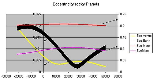
Plot of the changing orbital eccentricity of Mercury, Venus, Earth, and Mars over the next 50000 years. The arrows indicate the different scales used, as the eccentricities of Mercury and Mars are much greater than those of Venus and Earth. The 0 point on this plot is the year 2007.

Eccentricities of Solar System bodies

Object	eccentricity
Triton	0.00002
Venus	0.0068
Neptune	0.0086
Earth	0.0167
Titan	0.0288
Uranus	0.0472
Jupiter	0.0484
Saturn	0.0541
Moon	0.0549
1 Ceres	0.0758
4 Vesta	0.0887
Mars	0.0934
10 Hygiea	0.1146
Makemake	0.1559
Haumea	0.1887
Mercury	0.2056
2 Pallas	0.2313
Pluto	0.2488
3 Juno	0.2555
324 Bamberga	0.3400
Eris	0.4407
Nereid	0.7507
Sedna	0.8549
Halley's Comet	0.9671
Comet Hale-Bopp	0.9951
Comet Ikeya-Seki	0.9999
C/1980 E1	1.057
ʻOumuamua	1.20 [lower-alpha 1]
2I/Borisov	3.5 [lower-alpha 2]

The eccentricity of Earth's orbit is currently about 0.0167; its orbit is nearly circular. Venus and Neptune have even lower eccentricities. Over hundreds of thousands of years, the eccentricity of the Earth's orbit varies from nearly 0.0034 to almost 0.058 as a result of gravitational attractions among the planets. ^[3]

The table lists the values for all planets and dwarf planets, and selected asteroids, comets, and moons. Mercury has the greatest orbital eccentricity of any planet in the Solar System (e = 0.2056). Such eccentricity is sufficient for Mercury to receive twice as much solar irradiation at perihelion compared to aphelion. Before its demotion from planet status in 2006, Pluto was considered to be the planet with the most eccentric orbit (e = 0.248). Other Trans-Neptunian objects have significant eccentricity, notably the dwarf planet Eris (0.44). Even further out, Sedna, has an extremely-high eccentricity of 0.855 due to its estimated aphelion of 937 AU and perihelion of about 76 AU.

Most of the Solar System's asteroids have orbital eccentricities between 0 and 0.35 with an average value of 0.17. ^[4] Their comparatively high eccentricities are probably due to the influence of Jupiter and to past collisions.

The Moon's value is 0.0549, the most eccentric of the large moons of the Solar System. The four Galilean moons have an eccentricity of less than 0.01. Neptune's largest moon Triton has an eccentricity of 1.6×10⁻⁵ (0.000016), ^[5] the smallest eccentricity of any known moon in the Solar System;^{[ citation needed ]} its orbit is as close to a perfect circle as can be currently^{[ when? ]} measured. However, smaller moons, particularly irregular moons, can have significant eccentricity, such as Neptune's third largest moon Nereid (0.75).

Comets have very different values of eccentricity. Periodic comets have eccentricities mostly between 0.2 and 0.7, ^[6] but some of them have highly eccentric elliptical orbits with eccentricities just below 1; for example, Halley's Comet has a value of 0.967. Non-periodic comets follow near-parabolic orbits and thus have eccentricities even closer to 1. Examples include Comet Hale–Bopp with a value of 0.995 ^[7] and comet C/2006 P1 (McNaught) with a value of 1.000019. ^[8] As Hale–Bopp's value is less than 1, its orbit is elliptical and it will return. ^[7] Comet McNaught has a hyperbolic orbit while within the influence of the planets, ^[8] but is still bound to the Sun with an orbital period of about 10⁵ years. ^[9] Comet C/1980 E1 has the largest eccentricity of any known hyperbolic comet of solar origin with an eccentricity of 1.057, ^[10] and will eventually leave the Solar System.

ʻOumuamua is the first interstellar object found passing through the Solar System. Its orbital eccentricity of 1.20 indicates that ʻOumuamua has never been gravitationally bound to the Sun. It was discovered 0.2 AU (30000000 km; 19000000 mi) from Earth and is roughly 200 meters in diameter. It has an interstellar speed (velocity at infinity) of 26.33 km/s (58900 mph).

Mean eccentricity

The mean eccentricity of an object is the average eccentricity as a result of perturbations over a given time period. Neptune currently has an instant (current epoch) eccentricity of 0.0113, ^[11] but from 1800 to 2050 has a mean eccentricity of 0.00859. ^[12]

Climatic effect

Orbital mechanics require that the duration of the seasons be proportional to the area of Earth's orbit swept between the solstices and equinoxes, so when the orbital eccentricity is extreme, the seasons that occur on the far side of the orbit (aphelion) can be substantially longer in duration. Northern hemisphere autumn and winter occur at closest approach (perihelion), when Earth is moving at its maximum velocity—while the opposite occurs in the southern hemisphere. As a result, in the northern hemisphere, autumn and winter are slightly shorter than spring and summer—but in global terms this is balanced with them being longer below the equator. In 2006, the northern hemisphere summer was 4.66 days longer than winter, and spring was 2.9 days longer than autumn due to orbital eccentricity. ^{[13] [14]}

Apsidal precession also slowly changes the place in Earth's orbit where the solstices and equinoxes occur. This is a slow change in the orbit of Earth, not the axis of rotation, which is referred to as axial precession. The climatic effects of this change are part of the Milankovitch cycles. Over the next 10000 years, the northern hemisphere winters will become gradually longer and summers will become shorter. However, any cooling effect in one hemisphere is balanced by warming in the other, and any overall change will be counteracted by the fact that the eccentricity of Earth's orbit will be almost halved. ^[15] This will reduce the mean orbital radius and raise temperatures in both hemispheres closer to the mid-interglacial peak.

Exoplanets

Of the many exoplanets discovered, most have a higher orbital eccentricity than planets in the Solar System. Exoplanets found with low orbital eccentricity (near-circular orbits) are very close to their star and are tidally-locked to the star. All eight planets in the Solar System have near-circular orbits. The exoplanets discovered show that the Solar System, with its unusually-low eccentricity, is rare and unique. ^[16] One theory attributes this low eccentricity to the high number of planets in the Solar System; another suggests it arose because of its unique asteroid belts. A few other multiplanetary systems have been found, but none resemble the Solar System. The Solar System has unique planetesimal systems, which led the planets to have near-circular orbits. Solar planetesimal systems include the asteroid belt, Hilda family, Kuiper belt, Hills cloud, and the Oort cloud. The exoplanet systems discovered have either no planetesimal systems or a very large one. Low eccentricity is needed for habitability, especially advanced life. ^[17] High multiplicity planet systems are much more likely to have habitable exoplanets. ^{[18] [19]} The grand tack hypothesis of the Solar System also helps understand its near-circular orbits and other unique features. ^{[20] [21] [22] [23] [24] [25] [26] [27]}

See also

• Equation of time

Footnotes

1. ʻOumuamua was never bound to the Sun, so its orbit is hyperbolic: e ≈ 1.20 > 1 .
2. C/2019 Q4 (Borisov) was never bound to the Sun, so its orbit is hyperbolic: e ≈ 3.5 >> 1 .

References

1. Abraham, Ralph (2008). Foundations of mechanics. Jerrold E. Marsden (2nd ed.). Providence, R.I.: AMS Chelsea Pub./American Mathematical Society. ISBN   978-0-8218-4438-0. OCLC   191847156.
2. Bate, Roger R.; Mueller, Donald D.; White, Jerry E.; Saylor, William W. (2020). Fundamentals of Astrodynamics. Courier Dover. ISBN   978-0-486-49704-4 . Retrieved 4 March 2022.
3. A. Berger & M.F. Loutre (1991). "Graph of the eccentricity of the Earth's orbit". Illinois State Museum (Insolation values for the climate of the last 10 million years). Archived from the original on 6 January 2018.
4. Asteroids Archived 4 March 2007 at the Wayback Machine
5. David R. Williams (22 January 2008). "Neptunian Satellite Fact Sheet". NASA.
6. Lewis, John (2 December 2012). Physics and Chemistry of the Solar System. Academic Press. ISBN   9780323145848.
7. "JPL Small-Body Database Browser: C/1995 O1 (Hale-Bopp)" (2007-10-22 last obs). Retrieved 5 December 2008.
8. "JPL Small-Body Database Browser: C/2006 P1 (McNaught)" (2007-07-11 last obs). Retrieved 17 December 2009.
9. "Comet C/2006 P1 (McNaught) – facts and figures". Perth Observatory in Australia. 22 January 2007. Archived from the original on 18 February 2011.
10. "JPL Small-Body Database Browser: C/1980 E1 (Bowell)" (1986-12-02 last obs). Retrieved 22 March 2010.
11. Williams, David R. (29 November 2007). "Neptune Fact Sheet". NASA.
12. "Keplerian elements for 1800 A.D. to 2050 A.D." JPL Solar System Dynamics. Retrieved 17 December 2009.
13. Data from United States Naval Observatory Archived 13 October 2007 at the Wayback Machine
14. Berger A.; Loutre M.F.; Mélice J.L. (2006). "Equatorial insolation: from precession harmonics to eccentricity frequencies" (PDF). Clim. Past Discuss. 2 (4): 519–533. doi: 10.5194/cpd-2-519-2006 .
15. "Long Term Climate". ircamera.as.arizona.edu. Archived from the original on 2 June 2015. Retrieved 1 September 2016.
16. "ECCENTRICITY". exoplanets.org.
17. Ward, Peter; Brownlee, Donald (2000). Rare Earth: Why Complex Life is Uncommon in the Universe. Springer. pp. 122–123. ISBN   0-387-98701-0.
18. Limbach, MA; Turner, EL (2015). "Exoplanet orbital eccentricity: multiplicity relation and the Solar System". Proc Natl Acad Sci U S A. 112 (1): 20–4. arXiv: 1404.2552 . Bibcode:2015PNAS..112...20L. doi: 10.1073/pnas.1406545111 . PMC   4291657 . PMID   25512527.
19. Youdin, Andrew N.; Rieke, George H. (15 December 2015). "Planetesimals in Debris Disks". arXiv: 1512.04996 .{{cite journal}}: Cite journal requires |journal= (help)
20. Zubritsky, Elizabeth. "Jupiter's Youthful Travels Redefined Solar System". NASA . Retrieved 4 November 2015.
21. Sanders, Ray (23 August 2011). "How Did Jupiter Shape Our Solar System?". Universe Today . Retrieved 4 November 2015.
22. Choi, Charles Q. (23 March 2015). "Jupiter's 'Smashing' Migration May Explain Our Oddball Solar System". Space.com. Retrieved 4 November 2015.
23. Davidsson, Dr. Björn J. R. (9 March 2014). "Mysteries of the asteroid belt". The History of the Solar System. Retrieved 7 November 2015.
24. Raymond, Sean (2 August 2013). "The Grand Tack". PlanetPlanet. Retrieved 7 November 2015.
25. O'Brien, David P.; Walsh, Kevin J.; Morbidelli, Alessandro; Raymond, Sean N.; Mandell, Avi M. (2014). "Water delivery and giant impacts in the 'Grand Tack' scenario". Icarus. 239: 74–84. arXiv: 1407.3290 . Bibcode:2014Icar..239...74O. doi:10.1016/j.icarus.2014.05.009. S2CID   51737711.
26. Loeb, Abraham; Batista, Rafael; Sloan, David (August 2016). "Relative Likelihood for Life as a Function of Cosmic Time". Journal of Cosmology and Astroparticle Physics. 2016 (8): 040. arXiv: 1606.08448 . Bibcode:2016JCAP...08..040L. doi:10.1088/1475-7516/2016/08/040. S2CID   118489638.
27. "Is Earthly Life Premature from a Cosmic Perspective?". Harvard-Smithsonian Center for Astrophysics. 1 August 2016.

Further reading

• Prussing, John E.; Conway, Bruce A. (1993). Orbital Mechanics . New York: Oxford University Press. ISBN   0-19-507834-9.

External links

• World of Physics: Eccentricity
• The NOAA page on Climate Forcing Data includes (calculated) data from Berger (1978), Berger and Loutre (1991) ^{[ permanent dead link ]}. Laskar et al. (2004) on Earth orbital variations, Includes eccentricity over the last 50 million years and for the coming 20 million years.
• The orbital simulations by Varadi, Ghil and Runnegar (2003) provides series for Earth orbital eccentricity and orbital inclination.
• Kepler's Second law's simulation