Shape optimization

Last updated May 16, 2022

Shape optimization is part of the field of optimal control theory. The typical problem is to find the shape which is optimal in that it minimizes a certain cost functional while satisfying given constraints. In many cases, the functional being solved depends on the solution of a given partial differential equation defined on the variable domain.

Topology optimization is, in addition, concerned with the number of connected components/boundaries belonging to the domain. Such methods are needed since typically shape optimization methods work in a subset of allowable shapes which have fixed topological properties, such as having a fixed number of holes in them. Topological optimization techniques can then help work around the limitations of pure shape optimization.

Definition

Mathematically, shape optimization can be posed as the problem of finding a bounded set $\Omega$ , minimizing a functional

{\mathcal {F}}(\Omega )

,

possibly subject to a constraint of the form

{\mathcal {G}}(\Omega )=0.

Usually we are interested in sets $\Omega$ which are Lipschitz or C¹ boundary and consist of finitely many components, which is a way of saying that we would like to find a rather pleasing shape as a solution, not some jumble of rough bits and pieces. Sometimes additional constraints need to be imposed to that end to ensure well-posedness of the problem and uniqueness of the solution.

Shape optimization is an infinite-dimensional optimization problem. Furthermore, the space of allowable shapes over which the optimization is performed does not admit a vector space structure, making application of traditional optimization methods more difficult.

Examples

Among all three-dimensional shapes of given volume, find the one which has minimal surface area. Here:
${\mathcal {F}}(\Omega )={\mbox{Area}}(\partial \Omega )$ ,
with
${\mathcal {G}}(\Omega )={\mbox{Volume}}(\Omega )={\mbox{const.}}$
The answer, given by the isoperimetric inequality, is a ball.
Find the shape of an airplane wing which minimizes drag. Here the constraints could be the wing strength, or the wing dimensions.
Find the shape of various mechanical structures, which can resist a given stress while having a minimal mass/volume.
Given a known three-dimensional object with a fixed radiation source inside, deduce the shape and size of the source based on measurements done on part of the boundary of the object. A formulation of this inverse problem using least-squares fit leads to a shape optimization problem.

Techniques

Shape optimization problems are usually solved numerically, by using iterative methods. That is, one starts with an initial guess for a shape, and then gradually evolves it, until it morphs into the optimal shape.

Keeping track of the shape

To solve a shape optimization problem, one needs to find a way to represent a shape in the computer memory, and follow its evolution. Several approaches are usually used.

One approach is to follow the boundary of the shape. For that, one can sample the shape boundary in a relatively dense and uniform manner, that is, to consider enough points to get a sufficiently accurate outline of the shape. Then, one can evolve the shape by gradually moving the boundary points. This is called the Lagrangian approach.

Another approach is to consider a function defined on a rectangular box around the shape, which is positive inside of the shape, zero on the boundary of the shape, and negative outside of the shape. One can then evolve this function instead of the shape itself. One can consider a rectangular grid on the box and sample the function at the grid points. As the shape evolves, the grid points do not change; only the function values at the grid points change. This approach, of using a fixed grid, is called the Eulerian approach. The idea of using a function to represent the shape is at the basis of the level-set method.

A third approach is to think of the shape evolution as of a flow problem. That is, one can imagine that the shape is made of a plastic material gradually deforming such that any point inside or on the boundary of the shape can be always traced back to a point of the original shape in a one-to-one fashion. Mathematically, if $\Omega _{0}$ is the initial shape, and $\Omega _{t}$ is the shape at time t, one considers the diffeomorphisms

f_{t}:\Omega _{0}\to \Omega _{t},{\mbox{ for }}0\leq t\leq t_{0}.

The idea is again that shapes are difficult entities to be dealt with directly, so manipulate them by means of a function.

Iterative methods using shape gradients

Consider a smooth velocity field $V$ and the family of transformations $T_{s}$ of the initial domain $\Omega _{0}$ under the velocity field $V$ :

x(0)=x_{0}\in \Omega _{0},\quad x'(s)=V(x(s)),\quad T_{s}(x_{0})=x(s),\quad s\geq 0

,

and denote

\Omega _{0}\mapsto T_{s}(\Omega _{0})=\Omega _{s}.

Then the Gâteaux or shape derivative of ${\mathcal {F}}(\Omega )$ at $\Omega _{0}$ with respect to the shape is the limit of

d{\mathcal {F}}(\Omega _{0};V)=\lim _{s\to 0}{\frac {{\mathcal {F}}(\Omega _{s})-{\mathcal {F}}(\Omega _{0})}{s}}

if this limit exists. If in addition the derivative is linear with respect to $V$ , there is a unique element of $\nabla {\mathcal {F}}\in L^{2}(\partial \Omega _{0})$ and

d{\mathcal {F}}(\Omega _{0};V)=\langle \nabla {\mathcal {F}},V\rangle _{\partial \Omega _{0}}

where $\nabla {\mathcal {F}}$ is called the shape gradient. This gives a natural idea of gradient descent, where the boundary $\partial \Omega$ is evolved in the direction of negative shape gradient in order to reduce the value of the cost functional. Higher order derivatives can be similarly defined, leading to Newtonlike methods.

Typically, gradient descent is preferred, even if requires a large number of iterations, because, it can be hard to compute the second-order derivative (that is, the Hessian) of the objective functional ${\mathcal {F}}$ .

If the shape optimization problem has constraints, that is, the functional ${\mathcal {G}}$ is present, one has to find ways to convert the constrained problem into an unconstrained one. Sometimes ideas based on Lagrange multipliers, like the adjoint state method, can work.

Geometry parametrization

Shape optimization can be faced using standard optimization methods if a parametrization of the geometry is defined. Such parametrization is very important in CAE field where goal functions are usually complex functions evaluated using numerical models (CFD, FEA,...). A convenient approach, suitable for a wide class of problems, consists in the parametrization of the CAD model coupled with a full automation of all the process required for function evaluation (meshing, solving and result processing). Mesh morphing is a valid choice for complex problems that resolves typical issues associated with re-meshing such as discontinuities in the computed objective and constraint functions .^[1] In this case the parametrization is defined after the meshing stage acting directly on the numerical model used for calculation that is changed using mesh updating methods. There are several algorithms available for mesh morphing (deforming volumes, pseudosolids, radial basis functions). The selection of the parametrization approach depends mainly on the size of the problem: the CAD approach is preferred for small-to-medium sized models whilst the mesh morphing approach is the best (and sometimes the only feasible one) for large and very large models. The multi-objective Pareto optimization (NSGA II) could be utilized as a powerful approach for shape optimization. In this regard, the Pareto optimization approach displays useful advantages in design method such as the effect of area constraint that other multi-objective optimization cannot declare it. The approach of using a penalty function is an effective technique which could be used in the first stage of optimization. In this method the constrained shape design problem is adapted to an unconstrained problem with utilizing the constraints in the objective function as a penalty factor. Most of the time penalty factor is dependent to the amount of constraint variation rather than constraint number. The GA real-coded technique is applied in the present optimization problem. Therefore, the calculations are based on real value of variables. ^[2]

Related Research Articles

In mathematical optimization, the method of Lagrange multipliers is a strategy for finding the local maxima and minima of a function subject to equality constraints. It is named after the mathematician Joseph-Louis Lagrange. The basic idea is to convert a constrained problem into a form such that the derivative test of an unconstrained problem can still be applied. The relationship between the gradient of the function and gradients of the constraints rather naturally leads to a reformulation of the original problem, known as the Lagrangian function.

H_∞methods are used in control theory to synthesize controllers to achieve stabilization with guaranteed performance. To use H_∞ methods, a control designer expresses the control problem as a mathematical optimization problem and then finds the controller that solves this optimization. H_∞ techniques have the advantage over classical control techniques in that H_∞ techniques are readily applicable to problems involving multivariate systems with cross-coupling between channels; disadvantages of H_∞ techniques include the level of mathematical understanding needed to apply them successfully and the need for a reasonably good model of the system to be controlled. It is important to keep in mind that the resulting controller is only optimal with respect to the prescribed cost function and does not necessarily represent the best controller in terms of the usual performance measures used to evaluate controllers such as settling time, energy expended, etc. Also, non-linear constraints such as saturation are generally not well-handled. These methods were introduced into control theory in the late 1970s-early 1980s by George Zames, J. William Helton , and Allen Tannenbaum.

In mathematical analysis, a function of bounded variation, also known as $BV$ function, is a real-valued function whose total variation is bounded (finite): the graph of a function having this property is well behaved in a precise sense. For a continuous function of a single variable, being of bounded variation means that the distance along the direction of the $y$ -axis, neglecting the contribution of motion along $x$ -axis, traveled by a point moving along the graph has a finite value. For a continuous function of several variables, the meaning of the definition is the same, except for the fact that the continuous path to be considered cannot be the whole graph of the given function, but can be every intersection of the graph itself with a hyperplane parallel to a fixed $x$ -axis and to the $y$ -axis.

Global optimization is a branch of applied mathematics and numerical analysis that attempts to find the global minima or maxima of a function or a set of functions on a given set. It is usually described as a minimization problem because the maximization of the real-valued function $is equivalent to the minimization of the function .$

Topology optimization is a mathematical method that optimizes material layout within a given design space, for a given set of loads, boundary conditions and constraints with the goal of maximizing the performance of the system. Topology optimization is different from shape optimization and sizing optimization in the sense that the design can attain any shape within the design space, instead of dealing with predefined configurations.

Geometry processing, or mesh processing, is an area of research that uses concepts from applied mathematics, computer science and engineering to design efficient algorithms for the acquisition, reconstruction, analysis, manipulation, simulation and transmission of complex 3D models. As the name implies, many of the concepts, data structures, and algorithms are directly analogous to signal processing and image processing. For example, where image smoothing might convolve an intensity signal with a blur kernel formed using the Laplace operator, geometric smoothing might be achieved by convolving a surface geometry with a blur kernel formed using the Laplace-Beltrami operator.

In mathematics, a flow formalizes the idea of the motion of particles in a fluid. Flows are ubiquitous in science, including engineering and physics. The notion of flow is basic to the study of ordinary differential equations. Informally, a flow may be viewed as a continuous motion of points over time. More formally, a flow is a group action of the real numbers on a set.

In mathematics, more particularly in functional analysis, differential topology, and geometric measure theory, a k-current in the sense of Georges de Rham is a functional on the space of compactly supported differential k-forms, on a smooth manifold M. Currents formally behave like Schwartz distributions on a space of differential forms, but in a geometric setting, they can represent integration over a submanifold, generalizing the Dirac delta function, or more generally even directional derivatives of delta functions (multipoles) spread out along subsets of M.

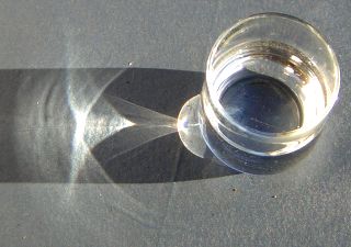
In optics, a caustic or caustic network is the envelope of light rays reflected or refracted by a curved surface or object, or the projection of that envelope of rays on another surface. The caustic is a curve or surface to which each of the light rays is tangent, defining a boundary of an envelope of rays as a curve of concentrated light. Therefore, in the photo to the right, caustics can be seen as patches of light or their bright edges. These shapes often have cusp singularities.

In mathematics and its applications, the signed distance function of a set Ω in a metric space determines the distance of a given point x from the boundary of Ω, with the sign determined by whether x is in Ω. The function has positive values at points x inside Ω, it decreases in value as x approaches the boundary of Ω where the signed distance function is zero, and it takes negative values outside of Ω. However, the alternative convention is also sometimes taken instead.

In mathematics, Bochner spaces are a generalization of the concept of $spaces$ to functions whose values lie in a Banach space which is not necessarily the space $or of real or complex numbers.$

Linear Programming Boosting (LPBoost) is a supervised classifier from the boosting family of classifiers. LPBoost maximizes a margin between training samples of different classes and hence also belongs to the class of margin-maximizing supervised classification algorithms. Consider a classification function

The topological derivative is, conceptually, a derivative of a shape functional with respect to infinitesimal changes in its topology, such as adding an infinitesimal hole or crack. When used in higher dimensions than one, the term topological gradient is also used to name the first-order term of the topological asymptotic expansion, dealing only with infinitesimal singular domain perturbations. It has applications in shape optimization, topology optimization, image processing and mechanical modeling.

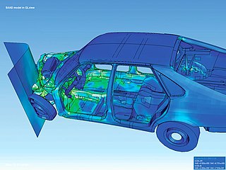
The finite element method (FEM) is a popular method for numerically solving differential equations arising in engineering and mathematical modeling. Typical problem areas of interest include the traditional fields of structural analysis, heat transfer, fluid flow, mass transport, and electromagnetic potential.

The adjoint state method is a numerical method for efficiently computing the gradient of a function or operator in a numerical optimization problem. It has applications in geophysics, seismic imaging, photonics and more recently in neural networks.

In mathematics, a free boundary problem is a partial differential equation to be solved for both an unknown function $and an unknown domain . The segment of the boundary of which is not known at the outset of the problem is the free boundary .$

The closest point method (CPM) is an embedding method for solving partial differential equations on surfaces. The closest point method uses standard numerical approaches such as finite differences, finite element or spectral methods in order to solve the embedding partial differential equation (PDE) which is equal to the original PDE on the surface. The solution is computed in a band surrounding the surface in order to be computationally efficient. In order to extend the data off the surface, the closest point method uses a closest point representation. This representation extends function values to be constant along directions normal to the surface.

In mathematics, the walk-on-spheres method (WoS) is a numerical probabilistic algorithm, or Monte-Carlo method, used mainly in order to approximate the solutions of some specific boundary value problem for partial differential equations (PDEs). The WoS method was first introduced by Mervin E. Muller in 1956 to solve Laplace's equation, and was since then generalized to other problems.

YaDICs is a program written to perform digital image correlation on 2D and 3D tomographic images. The program was designed to be both modular, by its plugin strategy and efficient, by it multithreading strategy. It incorporates different transformations, optimizing strategy, Global and/or local shape functions ...

In numerical mathematics, the gradient discretisation method (GDM) is a framework which contains classical and recent numerical schemes for diffusion problems of various kinds: linear or non-linear, steady-state or time-dependent. The schemes may be conforming or non-conforming, and may rely on very general polygonal or polyhedral meshes.

References

↑ Wilke, D.N.; Kok, S.; Groenwold, A.A. (2010) The application of gradient-only optimization methods for problems discretized using non-constant methods. Structural and Multidisciplinary Optimization, Vol. 40, 433-451.
↑ Talebitooti, R.; shojaeefard, M.H.; Yarmohammadisatri, Sadegh (2015). "Shape design optimization of cylindrical tank using b-spline curves". Computer & Fluids. 109: 100–112. doi:10.1016/j.compfluid.2014.12.004.

Sources

Allaire, G. (2002) Shape optimization by the homogenization method. Applied Mathematical Sciences 146, Springer Verlag. ISBN 0-387-95298-5
Ashok D. Belegundu, Tirupathi R. Chandrupatla. (2003) Optimization Concepts and applications in Engineering Prentice Hall. ISBN 0-13-031279-7.
Bendsøe M. P.; Sigmund O. (2003) Topology Optimization: Theory, Methods and Applications. Springer. ISBN 3-540-42992-1.
Burger, M.; Osher, S.L. (2005) A Survey on Level Set Methods for Inverse Problems and Optimal Design. European Journal of Applied Mathematics, vol.16 pp. 263–301.
Delfour, M.C.; Zolesio, J.-P. (2001) Shapes and Geometries - Analysis, Differential Calculus, and Optimization. SIAM. ISBN 0-89871-489-3.
Haslinger, J.; Mäkinen, R. (2003) Introduction to Shape Optimization: Theory, Approximation and Computation. Society for Industrial and Applied Mathematic. ISBN 0-89871-536-9.
Laporte, E.; Le Tallec, P. (2003) Numerical Methods in Sensitivity Analysis and Shape Optimization. Birkhäuser. ISBN 0-8176-4322-2.
Mohammadi, B.; Pironneau, O. (2001) Applied Shape Optimization for Fluids. Oxford University Press. ISBN 0-19-850743-7.
Simon J. (1980) Differentiation with respect to the domain in boundary value problems. Numer. Fuct. Anal. and Optimiz., 2(7&8), 649-687 (1980).

External links

Optopo Group — Simulations and bibliography of the optopo group at Ecole Polytechnique (France). Homogenization method and level set method.

This page is based on this Wikipedia article
Text is available under the CC BY-SA 4.0 license; additional terms may apply.
Images, videos and audio are available under their respective licenses.

[wilke-1] Wilke, D.N.; Kok, S.; Groenwold, A.A. (2010) The application of gradient-only optimization methods for problems discretized using non-constant methods. Structural and Multidisciplinary Optimization, Vol. 40, 433-451.

[ssttds-2] Talebitooti, R.; shojaeefard, M.H.; Yarmohammadisatri, Sadegh (2015). "Shape design optimization of cylindrical tank using b-spline curves". Computer & Fluids. 109: 100–112. doi:10.1016/j.compfluid.2014.12.004.

[1]

[2]