Solid of revolution

Rotating a curve. The surface formed is a surface of revolution; it encloses a solid of revolution.

Solids of revolution (Matemateca Ime-Usp)

In geometry, a solid of revolution is a solid figure obtained by rotating a plane figure around some straight line (the axis of revolution ), which may not intersect the generatrix (except at its boundary). The surface created by this revolution and which bounds the solid is the surface of revolution .

Assuming that the curve does not cross the axis, the solid's volume is equal to the length of the circle described by the figure's centroid multiplied by the figure's area (Pappus's second centroid theorem).

A representative disc is a three-dimensional volume element of a solid of revolution. The element is created by rotating a line segment (of length w) around some axis (located r units away), so that a cylindrical volume of πr²w units is enclosed.

Finding the volume

Two common methods for finding the volume of a solid of revolution are the disc method and the shell method of integration. To apply these methods, it is easiest to draw the graph in question; identify the area that is to be revolved about the axis of revolution; determine the volume of either a disc-shaped slice of the solid, with thickness δx, or a cylindrical shell of width δx; and then find the limiting sum of these volumes as δx approaches 0, a value which may be found by evaluating a suitable integral. A more rigorous justification can be given by attempting to evaluate a triple integral in cylindrical coordinates with two different orders of integration.

Disc method

Disc integration about the y-axis

Main article: Disc integration

The disc method is used when the slice that was drawn is perpendicular to the axis of revolution; i.e. when integrating parallel to the axis of revolution.

The volume of the solid formed by rotating the area between the curves of f(y) and g(y) and the lines y = a and y = b about the y-axis is given by

$${\displaystyle V=\pi \int _{a}^{b}\left|f(y)^{2}-g(y)^{2}\right|\,dy\,.}$$

If g(y) = 0 (e.g. revolving an area between the curve and the y-axis), this reduces to:

$${\displaystyle V=\pi \int _{a}^{b}f(y)^{2}\,dy\,.}$$

The method can be visualized by considering a thin horizontal rectangle at y between f(y) on top and g(y) on the bottom, and revolving it about the y-axis; it forms a ring (or disc in the case that g(y) = 0), with outer radius f(y) and inner radius g(y). The area of a ring is π(R² − r²), where R is the outer radius (in this case f(y)), and r is the inner radius (in this case g(y)). The volume of each infinitesimal disc is therefore πf(y)²dy. The limit of the Riemann sum of the volumes of the discs between a and b becomes integral (1).

Assuming the applicability of Fubini's theorem and the multivariate change of variables formula, the disk method may be derived in a straightforward manner by (denoting the solid as D):

$${\displaystyle V=\iiint _{D}dV=\int _{a}^{b}\int _{g(z)}^{f(z)}\int _{0}^{2\pi }r\,d\theta \,dr\,dz=2\pi \int _{a}^{b}\int _{g(z)}^{f(z)}r\,dr\,dz=2\pi \int _{a}^{b}{\frac {1}{2}}r^{2}\Vert _{g(z)}^{f(z)}\,dz=\pi \int _{a}^{b}(f(z)^{2}-g(z)^{2})\,dz}$$

Cylinder method

Main article: Shell integration

Shell integration

The cylinder method is used when the slice that was drawn is parallel to the axis of revolution; i.e. when integrating perpendicular to the axis of revolution.

The volume of the solid formed by rotating the area between the curves of f(x) and g(x) and the lines x = a and x = b about the y-axis is given by

$${\displaystyle V=2\pi \int _{a}^{b}x|f(x)-g(x)|\,dx\,.}$$

If g(x) = 0 (e.g. revolving an area between curve and y-axis), this reduces to:

$${\displaystyle V=2\pi \int _{a}^{b}x|f(x)|\,dx\,.}$$

The method can be visualized by considering a thin vertical rectangle at x with height f(x) − g(x), and revolving it about the y-axis; it forms a cylindrical shell. The lateral surface area of a cylinder is 2πrh, where r is the radius (in this case x), and h is the height (in this case f(x) − g(x)). Summing up all of the surface areas along the interval gives the total volume.

This method may be derived with the same triple integral, this time with a different order of integration:

$${\displaystyle V=\iiint _{D}dV=\int _{a}^{b}\int _{g(r)}^{f(r)}\int _{0}^{2\pi }r\,d\theta \,dz\,dr=2\pi \int _{a}^{b}\int _{g(r)}^{f(r)}r\,dz\,dr=2\pi \int _{a}^{b}r(f(r)-g(r))\,dr.}$$

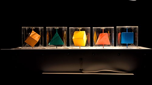
Solid of revolution demonstration

The shapes at rest

The shapes in motion, showing the solids of revolution formed by each

Parametric form

Mathematics and art: study of a vase as a solid of revolution by Paolo Uccello. 15th century

When a curve is defined by its parametric form (x(t),y(t)) in some interval [a,b], the volumes of the solids generated by revolving the curve around the x-axis or the y-axis are given by ^[1]

$${\displaystyle {\begin{aligned}V_{x}&=\int _{a}^{b}\pi y^{2}\,{\frac {dx}{dt}}\,dt\,,\\V_{y}&=\int _{a}^{b}\pi x^{2}\,{\frac {dy}{dt}}\,dt\,.\end{aligned}}}$$

Under the same circumstances the areas of the surfaces of the solids generated by revolving the curve around the x-axis or the y-axis are given by ^[2]

$${\displaystyle {\begin{aligned}A_{x}&=\int _{a}^{b}2\pi y\,{\sqrt {\left({\frac {dx}{dt}}\right)^{2}+\left({\frac {dy}{dt}}\right)^{2}}}\,dt\,,\\A_{y}&=\int _{a}^{b}2\pi x\,{\sqrt {\left({\frac {dx}{dt}}\right)^{2}+\left({\frac {dy}{dt}}\right)^{2}}}\,dt\,.\end{aligned}}}$$

This can also be derived from multivariable integration. If a plane curve is given by ${\displaystyle \langle x(t),y(t)\rangle }$ then its corresponding surface of revolution when revolved around the x-axis has Cartesian coordinates given by ${\displaystyle \mathbf {r} (t,\theta )=\langle y(t)\cos(\theta ),y(t)\sin(\theta ),x(t)\rangle }$ with ${\displaystyle 0\leq \theta \leq 2\pi }$. Then the surface area is given by the surface integral

$${\displaystyle A_{x}=\iint _{S}dS=\iint _{[a,b]\times [0,2\pi ]}\left\|{\frac {\partial \mathbf {r} }{\partial t}}\times {\frac {\partial \mathbf {r} }{\partial \theta }}\right\|\ d\theta \ dt=\int _{a}^{b}\int _{0}^{2\pi }\left\|{\frac {\partial \mathbf {r} }{\partial t}}\times {\frac {\partial \mathbf {r} }{\partial \theta }}\right\|\ d\theta \ dt.}$$

Computing the partial derivatives yields

$${\displaystyle {\frac {\partial \mathbf {r} }{\partial t}}=\left\langle {\frac {dy}{dt}}\cos(\theta ),{\frac {dy}{dt}}\sin(\theta ),{\frac {dx}{dt}}\right\rangle ,}$$

$${\displaystyle {\frac {\partial \mathbf {r} }{\partial \theta }}=\left\langle -y\sin(\theta ),y\cos(\theta ),0\right\rangle }$$

and computing the cross product yields

$${\displaystyle {\frac {\partial \mathbf {r} }{\partial t}}\times {\frac {\partial \mathbf {r} }{\partial \theta }}=\left\langle y\cos(\theta ){\frac {dx}{dt}},y\sin(\theta ){\frac {dx}{dt}},y{\frac {dy}{dt}}\right\rangle =y\left\langle \cos(\theta ){\frac {dx}{dt}},\sin(\theta ){\frac {dx}{dt}},{\frac {dy}{dt}}\right\rangle }$$

where the trigonometric identity ${\displaystyle \sin ^{2}(\theta )+\cos ^{2}(\theta )=1}$ was used. With this cross product, we get

$${\displaystyle {\begin{aligned}A_{x}&=\int _{a}^{b}\int _{0}^{2\pi }\left\|{\frac {\partial \mathbf {r} }{\partial t}}\times {\frac {\partial \mathbf {r} }{\partial \theta }}\right\|\ d\theta \ dt\\[1ex]&=\int _{a}^{b}\int _{0}^{2\pi }\left\|y\left\langle y\cos(\theta ){\frac {dx}{dt}},y\sin(\theta ){\frac {dx}{dt}},y{\frac {dy}{dt}}\right\rangle \right\|\ d\theta \ dt\\[1ex]&=\int _{a}^{b}\int _{0}^{2\pi }y{\sqrt {\cos ^{2}(\theta )\left({\frac {dx}{dt}}\right)^{2}+\sin ^{2}(\theta )\left({\frac {dx}{dt}}\right)^{2}+\left({\frac {dy}{dt}}\right)^{2}}}\ d\theta \ dt\\[1ex]&=\int _{a}^{b}\int _{0}^{2\pi }y{\sqrt {\left({\frac {dx}{dt}}\right)^{2}+\left({\frac {dy}{dt}}\right)^{2}}}\ d\theta \ dt\\[1ex]&=\int _{a}^{b}2\pi y{\sqrt {\left({\frac {dx}{dt}}\right)^{2}+\left({\frac {dy}{dt}}\right)^{2}}}\ dt\end{aligned}}}$$

where the same trigonometric identity was used again. The derivation for a surface obtained by revolving around the y-axis is similar.

Polar form

For a polar curve ${\displaystyle r=f(\theta )}$ where ${\displaystyle \alpha \leq \theta \leq \beta }$ and ${\displaystyle f(\theta )\geq 0}$, the volumes of the solids generated by revolving the curve around the x-axis or y-axis are

$${\displaystyle {\begin{aligned}V_{x}&=\int _{\alpha }^{\beta }\left(\pi r^{2}\sin ^{2}{\theta }\cos {\theta }\,{\frac {dr}{d\theta }}-\pi r^{3}\sin ^{3}{\theta }\right)d\theta \,,\\V_{y}&=\int _{\alpha }^{\beta }\left(\pi r^{2}\sin {\theta }\cos ^{2}{\theta }\,{\frac {dr}{d\theta }}+\pi r^{3}\cos ^{3}{\theta }\right)d\theta \,.\end{aligned}}}$$

The areas of the surfaces of the solids generated by revolving the curve around the x-axis or the y-axis are given

$${\displaystyle {\begin{aligned}A_{x}&=\int _{\alpha }^{\beta }2\pi r\sin {\theta }\,{\sqrt {r^{2}+\left({\frac {dr}{d\theta }}\right)^{2}}}\,d\theta \,,\\A_{y}&=\int _{\alpha }^{\beta }2\pi r\cos {\theta }\,{\sqrt {r^{2}+\left({\frac {dr}{d\theta }}\right)^{2}}}\,d\theta \,,\end{aligned}}}$$

See also

• Gabriel's Horn
• Guldinus theorem
• Pseudosphere
• Surface of revolution
• Ungula

Notes

1. Sharma, A. K. (2005). Application Of Integral Calculus. Discovery Publishing House. p. 168. ISBN   81-7141-967-4.
2. Singh, Ravish R. (1993). Engineering Mathematics (6th ed.). Tata McGraw-Hill. p. 6.90. ISBN   0-07-014615-2.

References

• "Volumes of Solids of Revolution". CliffsNotes.com. 12 Apr 2011. Archived from the original on 2012-03-19.
• Ayres, Frank; Mendelson, Elliott (2008). Calculus. Schaum's Outlines. McGraw-Hill Professional. pp. 244–248. ISBN   978-0-07-150861-2. ( online copy , p. 244, at Google Books)
• Weisstein, Eric W. "Solid of Revolution". MathWorld .