Confusingly, there are two different mathematical expressions in use, both called 'structure factor'. One is usually written ; it is more generally valid, and relates the observed diffracted intensity per atom to that produced by a single scattering unit. The other is usually written or and is only valid for systems with long-range positional order — crystals. This expression relates the amplitude and phase of the beam diffracted by the planes of the crystal ( are the Miller indices of the planes) to that produced by a single scattering unit at the vertices of the primitive unit cell. is not a special case of ; gives the scattering intensity, but gives the amplitude. It is the modulus squared that gives the scattering intensity. is defined for a perfect crystal, and is used in crystallography, while is most useful for disordered systems. For partially ordered systems such as crystalline polymers there is obviously overlap, and experts will switch from one expression to the other as needed.
The static structure factor is measured without resolving the energy of scattered photons/electrons/neutrons. Energy-resolved measurements yield the dynamic structure factor.
Derivation of S(q)
Consider the scattering of a beam of wavelength by an assembly of particles or atoms stationary at positions . Assume that the scattering is weak, so that the amplitude of the incident beam is constant throughout the sample volume (Born approximation), and absorption, refraction and multiple scattering can be neglected (kinematic diffraction). The direction of any scattered wave is defined by its scattering vector . , where and ( ) are the scattered and incident beam wavevectors, and is the angle between them. For elastic scattering, and , limiting the possible range of (see Ewald sphere). The amplitude and phase of this scattered wave will be the vector sum of the scattered waves from all the atoms [1][2]
For an assembly of atoms, is the atomic form factor of the -th atom. The scattered intensity is obtained by multiplying this function by its complex conjugate
(1)
The structure factor is defined as this intensity normalized by [3]
(2)
If all the atoms are identical, then Equation (1) becomes and so
(3)
Another useful simplification is if the material is isotropic, like a powder or a simple liquid. In that case, the intensity depends on and . In three dimensions, Equation (2) then simplifies to the Debye scattering equation:[1]
(4)
An alternative derivation gives good insight, but uses Fourier transforms and convolution. To be general, consider a scalar (real) quantity defined in a volume ; this may correspond, for instance, to a mass or charge distribution or to the refractive index of an inhomogeneous medium. If the scalar function is integrable, we can write its Fourier transform as . In the Born approximation the amplitude of the scattered wave corresponding to the scattering vector is proportional to the Fourier transform .[1] When the system under study is composed of a number of identical constituents (atoms, molecules, colloidal particles, etc.) each of which has a distribution of mass or charge then the total distribution can be considered the convolution of this function with a set of delta functions.
(5)
with the particle positions as before. Using the property that the Fourier transform of a convolution product is simply the product of the Fourier transforms of the two factors, we have , so that:
(6)
This is clearly the same as Equation (1) with all particles identical, except that here is shown explicitly as a function of .
In general, the particle positions are not fixed and the measurement takes place over a finite exposure time and with a macroscopic sample (much larger than the interparticle distance). The experimentally accessible intensity is thus an averaged one ; we need not specify whether denotes a time or ensemble average. To take this into account we can rewrite Equation (3) as:
(7)
Perfect crystals
In a crystal, the constitutive particles are arranged periodically, with translational symmetry forming a lattice. The crystal structure can be described as a Bravais lattice with a group of atoms, called the basis, placed at every lattice point; that is, [crystal structure] = [lattice] [basis]. If the lattice is infinite and completely regular, the system is a perfect crystal. For such a system, only a set of specific values for can give scattering, and the scattering amplitude for all other values is zero. This set of values forms a lattice, called the reciprocal lattice, which is the Fourier transform of the real-space crystal lattice.
In principle the scattering factor can be used to determine the scattering from a perfect crystal; in the simple case when the basis is a single atom at the origin (and again neglecting all thermal motion, so that there is no need for averaging) all the atoms have identical environments. Equation (1) can be written as
and .
The structure factor is then simply the squared modulus of the Fourier transform of the lattice, and shows the directions in which scattering can have non-zero intensity. At these values of the wave from every lattice point is in phase. The value of the structure factor is the same for all these reciprocal lattice points, and the intensity varies only due to changes in with .
Units
The units of the structure-factor amplitude depend on the incident radiation. For X-ray crystallography they are multiples of the unit of scattering by a single electron (2.82 m); for neutron scattering by atomic nuclei the unit of scattering length of m is commonly used.
The above discussion uses the wave vectors and . However, crystallography often uses wave vectors and . Therefore, when comparing equations from different sources, the factor may appear and disappear, and care to maintain consistent quantities is required to get correct numerical results.
Definition of Fhkl
In crystallography, the basis and lattice are treated separately. For a perfect crystal the lattice gives the reciprocal lattice, which determines the positions (angles) of diffracted beams, and the basis gives the structure factor which determines the amplitude and phase of the diffracted beams:
(8)
where the sum is over all atoms in the unit cell, are the positional coordinates of the -th atom, and is the scattering factor of the -th atom.[4] The coordinates have the directions and dimensions of the lattice vectors . That is, (0,0,0) is at the lattice point, the origin of position in the unit cell; (1,0,0) is at the next lattice point along and (1/2, 1/2, 1/2) is at the body center of the unit cell. defines a reciprocal lattice point at which corresponds to the real-space plane defined by the Miller indices (see Bragg's law).
is the vector sum of waves from all atoms within the unit cell. An atom at any lattice point has the reference phase angle zero for all since then is always an integer. A wave scattered from an atom at (1/2, 0, 0) will be in phase if is even, out of phase if is odd.
Again an alternative view using convolution can be helpful. Since [crystal structure] = [lattice] [basis], [crystal structure] = [lattice] [basis]; that is, scattering [reciprocal lattice] [structure factor].
Examples of Fhkl in 3-D
Body-centered cubic (BCC)
For the body-centered cubic Bravais lattice (cI), we use the points and which leads us to
and hence
Face-centered cubic (FCC)
The FCC lattice is a Bravais lattice, and its Fourier transform is a body-centered cubic lattice. However to obtain without this shortcut, consider an FCC crystal with one atom at each lattice point as a primitive or simple cubic with a basis of 4 atoms, at the origin and at the three adjacent face centers, , and . Equation (8) becomes
with the result
The most intense diffraction peak from a material that crystallizes in the FCC structure is typically the (111). Films of FCC materials like gold tend to grow in a (111) orientation with a triangular surface symmetry. A zero diffracted intensity for a group of diffracted beams (here, of mixed parity) is called a systematic absence.
Diamond crystal structure
The diamond cubic crystal structure occurs for example diamond (carbon), tin, and most semiconductors. There are 8 atoms in the cubic unit cell. We can consider the structure as a simple cubic with a basis of 8 atoms, at positions
But comparing this to the FCC above, we see that it is simpler to describe the structure as FCC with a basis of two atoms at (0, 0, 0) and (1/4, 1/4, 1/4). For this basis, Equation (8) becomes:
And then the structure factor for the diamond cubic structure is the product of this and the structure factor for FCC above, (only including the atomic form factor once)
with the result
If h, k, ℓ are of mixed parity (odd and even values combined) the first (FCC) term is zero, so
If h, k, ℓ are all even or all odd then the first (FCC) term is 4
if h+k+ℓ is odd then
if h+k+ℓ is even and exactly divisible by 4 () then
if h+k+ℓ is even but not exactly divisible by 4 () the second term is zero and
These points are encapsulated by the following equations:
where is an integer.
Zincblende crystal structure
The zincblende structure is similar to the diamond structure except that it is a compound of two distinct interpenetrating fcc lattices, rather than all the same element. Denoting the two elements in the compound by and , the resulting structure factor is
Cesium chloride
Cesium chloride is a simple cubic crystal lattice with a basis of Cs at (0,0,0) and Cl at (1/2, 1/2, 1/2) (or the other way around, it makes no difference). Equation (8) becomes
We then arrive at the following result for the structure factor for scattering from a plane :
and for scattered intensity,
Hexagonal close-packed (HCP)
In an HCP crystal such as graphite, the two coordinates include the origin and the next plane up the c axis located at c/2, and hence , which gives us
From this it is convenient to define dummy variable , and from there consider the modulus squared so hence
This leads us to the following conditions for the structure factor:
Perfect crystals in one and two dimensions
The reciprocal lattice is easily constructed in one dimension: for particles on a line with a period , the reciprocal lattice is an infinite array of points with spacing . In two dimensions, there are only five Bravais lattices. The corresponding reciprocal lattices have the same symmetry as the direct lattice. 2-D lattices are excellent for demonstrating simple diffraction geometry on a flat screen, as below. Equations (1)–(7) for structure factor apply with a scattering vector of limited dimensionality and a crystallographic structure factor can be defined in 2-D as .
However, recall that real 2-D crystals such as graphene exist in 3-D. The reciprocal lattice of a 2-D hexagonal sheet that exists in 3-D space in the plane is a hexagonal array of lines parallel to the or axis that extend to and intersect any plane of constant in a hexagonal array of points.
Diagram of scattering by a square (planar) lattice. The incident and outgoing beam are shown, as well as the relation between their wave vectors , and the scattering vector .
The Figure shows the construction of one vector of a 2-D reciprocal lattice and its relation to a scattering experiment.
A parallel beam, with wave vector is incident on a square lattice of parameter . The scattered wave is detected at a certain angle, which defines the wave vector of the outgoing beam, (under the assumption of elastic scattering, ). One can equally define the scattering vector and construct the harmonic pattern . In the depicted example, the spacing of this pattern coincides to the distance between particle rows: , so that contributions to the scattering from all particles are in phase (constructive interference). Thus, the total signal in direction is strong, and belongs to the reciprocal lattice. It is easily shown that this configuration fulfills Bragg's law.
Structure factor of a periodic chain, for different particle numbers .
Imperfect crystals
Technically a perfect crystal must be infinite, so a finite size is an imperfection. Real crystals always exhibit imperfections of their order besides their finite size, and these imperfections can have profound effects on the properties of the material. André Guinier[5] proposed a widely employed distinction between imperfections that preserve the long-range order of the crystal that he called disorder of the first kind and those that destroy it called disorder of the second kind. An example of the first is thermal vibration; an example of the second is some density of dislocations.
The generally applicable structure factor can be used to include the effect of any imperfection. In crystallography, these effects are treated as separate from the structure factor , so separate factors for size or thermal effects are introduced into the expressions for scattered intensity, leaving the perfect crystal structure factor unchanged. Therefore, a detailed description of these factors in crystallographic structure modeling and structure determination by diffraction is not appropriate in this article.
Finite-size effects
For a finite crystal means that the sums in equations 1-7 are now over a finite . The effect is most easily demonstrated with a 1-D lattice of points. The sum of the phase factors is a geometric series and the structure factor becomes:
This function is shown in the Figure for different values of . When the scattering from every particle is in phase, which is when the scattering is at a reciprocal lattice point , the sum of the amplitudes must be and so the maxima in intensity are . Taking the above expression for and estimating the limit using, for instance, L'Hôpital's rule) shows that as seen in the Figure. At the midpoint (by direct evaluation) and the peak width decreases like . In the large limit, the peaks become infinitely sharp Dirac delta functions, the reciprocal lattice of the perfect 1-D lattice.
In crystallography when is used, is large, and the formal size effect on diffraction is taken as , which is the same as the expression for above near to the reciprocal lattice points, . Using convolution, we can describe the finite real crystal structure as [lattice] [basis]rectangular function, where the rectangular function has a value 1 inside the crystal and 0 outside it. Then [crystal structure] = [lattice] [basis] [rectangular function]; that is, scattering [reciprocal lattice] [structure factor] [ sinc function]. Thus the intensity, which is a delta function of position for the perfect crystal, becomes a function around every point with a maximum , a width , area .
Disorder of the first kind
This model for disorder in a crystal starts with the structure factor of a perfect crystal. In one-dimension for simplicity and with N planes, we then start with the expression above for a perfect finite lattice, and then this disorder only changes by a multiplicative factor, to give[1]
where the disorder is measured by the mean-square displacement of the positions from their positions in a perfect one-dimensional lattice: , i.e., , where is a small (much less than ) random displacement. For disorder of the first kind, each random displacement is independent of the others, and with respect to a perfect lattice. Thus the displacements do not destroy the translational order of the crystal. This has the consequence that for infinite crystals () the structure factor still has delta-function Bragg peaks – the peak width still goes to zero as , with this kind of disorder. However, it does reduce the amplitude of the peaks, and due to the factor of in the exponential factor, it reduces peaks at large much more than peaks at small .
The structure is simply reduced by a and disorder dependent term because all disorder of the first-kind does is smear out the scattering planes, effectively reducing the form factor.
In three dimensions the effect is the same, the structure is again reduced by a multiplicative factor, and this factor is often called the Debye–Waller factor. Note that the Debye–Waller factor is often ascribed to thermal motion, i.e., the are due to thermal motion, but any random displacements about a perfect lattice, not just thermal ones, will contribute to the Debye–Waller factor.
Disorder of the second kind
However, fluctuations that cause the correlations between pairs of atoms to decrease as their separation increases, causes the Bragg peaks in the structure factor of a crystal to broaden. To see how this works, we consider a one-dimensional toy model: a stack of plates with mean spacing . The derivation follows that in chapter 9 of Guinier's textbook.[6] This model has been pioneered by and applied to a number of materials by Hosemann and collaborators[7] over a number of years. Guinier and they termed this disorder of the second kind, and Hosemann in particular referred to this imperfect crystalline ordering as paracrystalline ordering. Disorder of the first kind is the source of the Debye–Waller factor.
To derive the model we start with the definition (in one dimension) of the
To start with we will consider, for simplicity an infinite crystal, i.e., . We will consider a finite crystal with disorder of the second-type below.
For our infinite crystal, we want to consider pairs of lattice sites. For large each plane of an infinite crystal, there are two neighbours planes away, so the above double sum becomes a single sum over pairs of neighbours either side of an atom, at positions and lattice spacings away, times . So, then
where is the probability density function for the separation of a pair of planes, lattice spacings apart. For the separation of neighbouring planes we assume for simplicity that the fluctuations around the mean neighbour spacing of a are Gaussian, i.e., that
and we also assume that the fluctuations between a plane and its neighbour, and between this neighbour and the next plane, are independent. Then is just the convolution of two s, etc. As the convolution of two Gaussians is just another Gaussian, we have that
The sum in is then just a sum of Fourier transforms of Gaussians, and so
for . The sum is just the real part of the sum and so the structure factor of the infinite but disordered crystal is
This has peaks at maxima , where . These peaks have heights
i.e., the height of successive peaks drop off as the order of the peak (and so ) squared. Unlike finite-size effects that broaden peaks but do not decrease their height, disorder lowers peak heights. Note that here we assuming that the disorder is relatively weak, so that we still have relatively well defined peaks. This is the limit , where . In this limit, near a peak we can approximate , with and obtain
which is a Lorentzian or Cauchy function, of FWHM , i.e., the FWHM increases as the square of the order of peak, and so as the square of the wave vector at the peak.
Finally, the product of the peak height and the FWHM is constant and equals , in the limit. For the first few peaks where is not large, this is just the limit.
Finite crystals with disorder of the second kind
For a one-dimensional crystal of size
where the factor in parentheses comes from the fact the sum is over nearest-neighbour pairs (), next nearest-neighbours (), ... and for a crystal of planes, there are pairs of nearest neighbours, pairs of next-nearest neighbours, etc.
Liquids
In contrast with crystals, liquids have no long-range order (in particular, there is no regular lattice), so the structure factor does not exhibit sharp peaks. They do however show a certain degree of short-range order, depending on their density and on the strength of the interaction between particles. Liquids are isotropic, so that, after the averaging operation in Equation (4), the structure factor only depends on the absolute magnitude of the scattering vector . For further evaluation, it is convenient to separate the diagonal terms in the double sum, whose phase is identically zero, and therefore each contribute a unit constant:
In the limiting case of no interaction, the system is an ideal gas and the structure factor is completely featureless: , because there is no correlation between the positions and of different particles (they are independent random variables), so the off-diagonal terms in Equation (9) average to zero: .
High-q limit
Even for interacting particles, at high scattering vector the structure factor goes to 1. This result follows from Equation (10), since is the Fourier transform of the "regular" function and thus goes to zero for high values of the argument . This reasoning does not hold for a perfect crystal, where the distribution function exhibits infinitely sharp peaks.
Low-q limit
In the low- limit, as the system is probed over large length scales, the structure factor contains thermodynamic information, being related to the isothermal compressibility of the liquid by the compressibility equation:
.
Hard-sphere liquids
Structure factor of a hard-sphere fluid, calculated using the Percus-Yevick approximation, for volume fractions from 1% to 40%.
In the hard sphere model, the particles are described as impenetrable spheres with radius ; thus, their center-to-center distance and they experience no interaction beyond this distance. Their interaction potential can be written as:
This model has an analytical solution[9] in the Percus–Yevick approximation. Although highly simplified, it provides a good description for systems ranging from liquid metals[10] to colloidal suspensions.[11] In an illustration, the structure factor for a hard-sphere fluid is shown in the Figure, for volume fractions from 1% to 40%.
Polymers
In polymer systems, the general definition (4) holds; the elementary constituents are now the monomers making up the chains. However, the structure factor being a measure of the correlation between particle positions, one can reasonably expect that this correlation will be different for monomers belonging to the same chain or to different chains.
Let us assume that the volume contains identical molecules, each composed of monomers, such that ( is also known as the degree of polymerization). We can rewrite (4) as:
,
(11)
where indices label the different molecules and the different monomers along each molecule. On the right-hand side we separated intramolecular () and intermolecular () terms. Using the equivalence of the chains, (11) can be simplified:[12]
In physics, the cross section is a measure of the probability that a specific process will take place in a collision of two particles. For example, the Rutherford cross-section is a measure of probability that an alpha particle will be deflected by a given angle during an interaction with an atomic nucleus. Cross section is typically denoted σ (sigma) and is expressed in units of area, more specifically in barns. In a way, it can be thought of as the size of the object that the excitation must hit in order for the process to occur, but more exactly, it is a parameter of a stochastic process.
In physics, a phonon is a collective excitation in a periodic, elastic arrangement of atoms or molecules in condensed matter, specifically in solids and some liquids. A type of quasiparticle, a phonon is an excited state in the quantum mechanical quantization of the modes of vibrations for elastic structures of interacting particles. Phonons can be thought of as quantized sound waves, similar to photons as quantized light waves.
In physics, mean free path is the average distance over which a moving particle travels before substantially changing its direction or energy, typically as a result of one or more successive collisions with other particles.
In mathematics and physical science, spherical harmonics are special functions defined on the surface of a sphere. They are often employed in solving partial differential equations in many scientific fields. A list of the spherical harmonics is available in Table of spherical harmonics.
In condensed matter physics, Bloch's theorem states that solutions to the Schrödinger equation in a periodic potential can be expressed as plane waves modulated by periodic functions. The theorem is named after the Swiss physicist Felix Bloch, who discovered the theorem in 1929. Mathematically, they are written
In atomic physics, hyperfine structure is defined by small shifts in otherwise degenerate energy levels and the resulting splittings in those energy levels of atoms, molecules, and ions, due to electromagnetic multipole interaction between the nucleus and electron clouds.
In physics, the reciprocal lattice emerges from the Fourier transform of another lattice. The direct lattice or real lattice is a periodic function in physical space, such as a crystal system. The reciprocal lattice exists in the mathematical space of spatial frequencies, known as reciprocal space or k space, where refers to the wavevector.
In quantum physics, the scattering amplitude is the probability amplitude of the outgoing spherical wave relative to the incoming plane wave in a stationary-state scattering process. At large distances from the centrally symmetric scattering center, the plane wave is described by the wavefunction
Miller indices form a notation system in crystallography for lattice planes in crystal (Bravais) lattices.
In solid-state physics, the tight-binding model is an approach to the calculation of electronic band structure using an approximate set of wave functions based upon superposition of wave functions for isolated atoms located at each atomic site. The method is closely related to the LCAO method used in chemistry. Tight-binding models are applied to a wide variety of solids. The model gives good qualitative results in many cases and can be combined with other models that give better results where the tight-binding model fails. Though the tight-binding model is a one-electron model, the model also provides a basis for more advanced calculations like the calculation of surface states and application to various kinds of many-body problem and quasiparticle calculations.
The Debye–Waller factor (DWF), named after Peter Debye and Ivar Waller, is used in condensed matter physics to describe the attenuation of x-ray scattering or coherent neutron scattering caused by thermal motion. It is also called the B factor, atomic B factor, or temperature factor. Often, "Debye–Waller factor" is used as a generic term that comprises the Lamb–Mössbauer factor of incoherent neutron scattering and Mössbauer spectroscopy.
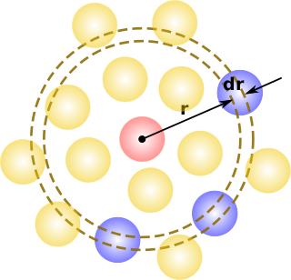
In statistical mechanics, the radial distribution function, in a system of particles, describes how density varies as a function of distance from a reference particle.
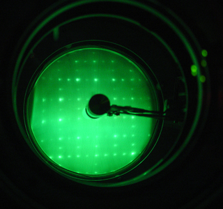
Low-energy electron diffraction (LEED) is a technique for the determination of the surface structure of single-crystalline materials by bombardment with a collimated beam of low-energy electrons (30–200 eV) and observation of diffracted electrons as spots on a fluorescent screen.
Ewald summation, named after Paul Peter Ewald, is a method for computing long-range interactions in periodic systems. It was first developed as the method for calculating the electrostatic energies of ionic crystals, and is now commonly used for calculating long-range interactions in computational chemistry. Ewald summation is a special case of the Poisson summation formula, replacing the summation of interaction energies in real space with an equivalent summation in Fourier space. In this method, the long-range interaction is divided into two parts: a short-range contribution, and a long-range contribution which does not have a singularity. The short-range contribution is calculated in real space, whereas the long-range contribution is calculated using a Fourier transform. The advantage of this method is the rapid convergence of the energy compared with that of a direct summation. This means that the method has high accuracy and reasonable speed when computing long-range interactions, and it is thus the de facto standard method for calculating long-range interactions in periodic systems. The method requires charge neutrality of the molecular system to accurately calculate the total Coulombic interaction. A study of the truncation errors introduced in the energy and force calculations of disordered point-charge systems is provided by Kolafa and Perram.
In crystallography and solid state physics, the Laue equations relate incoming waves to outgoing waves in the process of elastic scattering, where the photon energy or light temporal frequency does not change upon scattering by a crystal lattice. They are named after physicist Max von Laue (1879–1960).
In mathematics, vector spherical harmonics (VSH) are an extension of the scalar spherical harmonics for use with vector fields. The components of the VSH are complex-valued functions expressed in the spherical coordinate basis vectors.
The multislice algorithm is a method for the simulation of the elastic scattering of an electron beam with matter, including all multiple scattering effects. The method is reviewed in the book by John M. Cowley, and also the work by Ishizuka. The algorithm is used in the simulation of high resolution transmission electron microscopy (HREM) micrographs, and serves as a useful tool for analyzing experimental images. This article describes some relevant background information, the theoretical basis of the technique, approximations used, and several software packages that implement this technique. Some of the advantages and limitations of the technique and important considerations that need to be taken into account are described.
Static force fields are fields, such as a simple electric, magnetic or gravitational fields, that exist without excitations. The most common approximation method that physicists use for scattering calculations can be interpreted as static forces arising from the interactions between two bodies mediated by virtual particles, particles that exist for only a short time determined by the uncertainty principle. The virtual particles, also known as force carriers, are bosons, with different bosons associated with each force.
Partial-wave analysis, in the context of quantum mechanics, refers to a technique for solving scattering problems by decomposing each wave into its constituent angular-momentum components and solving using boundary conditions.
Heat transfer physics describes the kinetics of energy storage, transport, and energy transformation by principal energy carriers: phonons, electrons, fluid particles, and photons. Heat is thermal energy stored in temperature-dependent motion of particles including electrons, atomic nuclei, individual atoms, and molecules. Heat is transferred to and from matter by the principal energy carriers. The state of energy stored within matter, or transported by the carriers, is described by a combination of classical and quantum statistical mechanics. The energy is different made (converted) among various carriers. The heat transfer processes are governed by the rates at which various related physical phenomena occur, such as the rate of particle collisions in classical mechanics. These various states and kinetics determine the heat transfer, i.e., the net rate of energy storage or transport. Governing these process from the atomic level to macroscale are the laws of thermodynamics, including conservation of energy.
References
Als-Nielsen, N. and McMorrow, D. (2011). Elements of Modern X-ray Physics (2nd edition). John Wiley & Sons.
Guinier, A. (1963). X-ray Diffraction. In Crystals, Imperfect Crystals, and Amorphous Bodies. W. H. Freeman and Co.
This page is based on this Wikipedia article Text is available under the CC BY-SA 4.0 license; additional terms may apply. Images, videos and audio are available under their respective licenses.