Consider a localparametrisation of M. Let be an openneighbourhood of 0 with coordinates , and let be a smooth parametrisation of M in a neighbourhood of one of its points.
For a fixed the affine normal line to M at may be parametrised by t where
The affine focal set is given geometrically as the infinitesimalintersections of the n-parameter family of affine normal lines. To calculate, choose an affine normal line, say at point p; then look at the affine normal lines at points infinitesimally close to p and see if any intersect the one at p. If p is infinitesimally close to , then it may be expressed as where represents the infinitesimal difference. Thus and will be our p and its neighbour.
Solve for t and .
This can be done by using power series expansions, and is not too difficult; it is lengthy and has thus been omitted.
The solutions to are when 1/t is an eigenvalue of S and that is a corresponding eigenvector. The eigenvalues of S are not always distinct: there may be repeated roots, there may be complex roots, and S may not always be diagonalisable. For , where denotes the greatest integer function, there will generically be (n−2k)-pieces of the affine focal set above each point p. The −2k corresponds to pairs of eigenvalues becoming complex (like the solution to as a changes from negative to positive).
The affine focal set need not be made up of smooth hypersurfaces. In fact, for a generic hypersurface M, the affine focal set will have singularities. The singularities could be found by calculation, but that may be difficult, and there is no idea of what the singularity looks like up to diffeomorphism. Using singularity theory gives much more information.
Singularity theory approach
The idea here is to define a family of functions over M. The family will have the ambient real (n+1)-space as its parameter space, i.e. for each choice of ambient point there is function defined over M. This family is the family of affine distance functions:
Given an ambient point and a surface point p, it is possible to decompose the chord joining p to as a tangential component and a transverse component parallel to . The value of Δ is given implicitly in the equation
where Z is a tangent vector. Now, what is sought is the bifurcation set of the family Δ, i.e. the ambient points for which the restricted function
To discover if the Jacobian matrix has zero determinant, differentiating the equation x - p = Z + ΔA is needed. Let X be a tangent vector to M, and differentiate in that direction:
where I is the identity. This means that and . The last equality says that we have the following equation of differential one-forms. The Jacobian matrix will have zero determinant if, and only if, is degenerate as a one-form, i.e. for all tangent vectors X. Since it follows that is degenerate if, and only if, is degenerate. Since h is a non-degenerate two-form it follows that Z = 0. Notice that since M has a non-degenerate second fundamental form it follows that h is a non-degenerate two-form. Since Z = 0 the set of ambient points x for which the restricted function has a singularity at some p is the affine normal line to M at p.
To compute the Hessian matrix, consider the differential two-form . This is the two-form whose matrix representation is the Hessian matrix. It has already been seen that and that What remains is
.
Now assume that Δ has a singularity at p, i.e. Z = 0, then we have the two-form
.
It also has been seen that , and so the two-form becomes
.
This is degenerate as a two-form if, and only if, there exists non-zero X for which it is zero for all Y. Since h is non-degenerate it must be that and . So the singularity is degenerate if, and only if, the ambient point x lies on the affine normal line to p and the reciprocal of its distance from p is an eigenvalue of S, i.e. points where 1/t is an eigenvalue of S. The affine focal set!
Singular points
The affine focal set can be the following:
To find the singular points, simply differentiate p + tA in some tangent direction X:
The affine focal set is singular if, and only if, there exists non-zero X such that , i.e. if, and only if, X is an eigenvector of S and the derivative of t in that direction is zero. This means that the derivative of an affine principal curvature in its own affine principal direction is zero.
Local structure
Standard ideas can be used in singularity theory to classify, up to local diffeomorphism, the affine focal set. If the family of affine distance functions can be shown to be a certain kind of family then the local structure is known. The family of affine distance functions should be a versal unfolding of the singularities which arise.
The affine focal set of a plane curve will generically consist of smooth pieces of curve and ordinary cusp points (semi-cubical parabolae).
The question of the local structure in much higher dimension is of great interest. For example, it is possible to construct a discrete list of singularity types (up to local diffeomorphism). In much higher dimensions, no such discrete list can be constructed, as there are functional moduli.
Related Research Articles
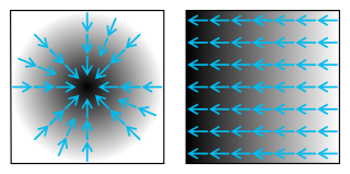
In vector calculus, the gradient of a scalar-valued differentiable function f of several variables is the vector field whose value at a point is the vector whose components are the partial derivatives of at . That is, for , its gradient is defined at the point in n-dimensional space as the vector:
In mathematics and physics, Laplace's equation is a second-order partial differential equation named after Pierre-Simon Laplace who first studied its properties. This is often written as
In mathematics, a quadric or quadric surface, is a generalization of conic sections. It is a hypersurface in a (D + 1)-dimensional space, and it is defined as the zero set of an irreducible polynomial of degree two in D + 1 variables. When the defining polynomial is not absolutely irreducible, the zero set is generally not considered a quadric, although it is often called a degenerate quadric or a reducible quadric.
In statistical mechanics, the Fokker–Planck equation is a partial differential equation that describes the time evolution of the probability density function of the velocity of a particle under the influence of drag forces and random forces, as in Brownian motion. The equation can be generalized to other observables as well. It is named after Adriaan Fokker and Max Planck, and is also known as the Kolmogorov forward equation, after Andrey Kolmogorov, who independently discovered the concept in 1931. When applied to particle position distributions, it is better known as the Smoluchowski equation, and in this context it is equivalent to the convection–diffusion equation. The case with zero diffusion is known in statistical mechanics as the Liouville equation. The Fokker–Planck equation is obtained from the master equation through Kramers–Moyal expansion.
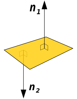
In geometry, a normal is an object such as a line, ray, or vector that is perpendicular to a given object. For example, the normal line to a plane curve at a given point is the (infinite) line perpendicular to the tangent line to the curve at the point. A normal vector may have length one or its length may represent the curvature of the object ; its algebraic sign may indicate sides.
In mathematics, the Laplace operator or Laplacian is a differential operator given by the divergence of the gradient of a function on Euclidean space. It is usually denoted by the symbols , , or . In a Cartesian coordinate system, the Laplacian is given by the sum of second partial derivatives of the function with respect to each independent variable. In other coordinate systems, such as cylindrical and spherical coordinates, the Laplacian also has a useful form. Informally, the Laplacian Δf(p) of a function f at a point p measures by how much the average value of f over small spheres or balls centered at p deviates from f(p).
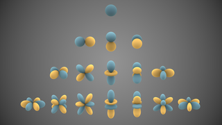
In mathematics and physical science, spherical harmonics are special functions defined on the surface of a sphere. They are often employed in solving partial differential equations in many scientific fields.
In Euclidean geometry, a translation is a geometric transformation that moves every point of a figure or a space by the same distance in a given direction. A translation can also be interpreted as the addition of a constant vector to every point, or as shifting the origin of the coordinate system. In a Euclidean space, any translation is an isometry.
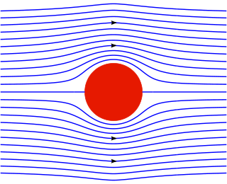
The stream function is defined for incompressible (divergence-free) flows in two dimensions – as well as in three dimensions with axisymmetry. The flow velocity components can be expressed as the derivatives of the scalar stream function. The stream function can be used to plot streamlines, which represent the trajectories of particles in a steady flow. The two-dimensional Lagrange stream function was introduced by Joseph Louis Lagrange in 1781. The Stokes stream function is for axisymmetrical three-dimensional flow, and is named after George Gabriel Stokes.
In vector calculus, Green's theorem relates a line integral around a simple closed curve C to a double integral over the plane region D bounded by C. It is the two-dimensional special case of Stokes' theorem.
In mathematics, an affine algebraic plane curve is the zero set of a polynomial in two variables. A projective algebraic plane curve is the zero set in a projective plane of a homogeneous polynomial in three variables. An affine algebraic plane curve can be completed in a projective algebraic plane curve by homogenizing its defining polynomial. Conversely, a projective algebraic plane curve of homogeneous equation h(x, y, t) = 0 can be restricted to the affine algebraic plane curve of equation h(x, y, 1) = 0. These two operations are each inverse to the other; therefore, the phrase algebraic plane curve is often used without specifying explicitly whether it is the affine or the projective case that is considered.
In the calculus of variations, a field of mathematical analysis, the functional derivative relates a change in a Functional to a change in a function on which the functional depends.
In mathematics, the Hessian matrix or Hessian is a square matrix of second-order partial derivatives of a scalar-valued function, or scalar field. It describes the local curvature of a function of many variables. The Hessian matrix was developed in the 19th century by the German mathematician Ludwig Otto Hesse and later named after him. Hesse originally used the term "functional determinants".
Scalar potential, simply stated, describes the situation where the difference in the potential energies of an object in two different positions depends only on the positions, not upon the path taken by the object in traveling from one position to the other. It is a scalar field in three-space: a directionless value (scalar) that depends only on its location. A familiar example is potential energy due to gravity.
In mathematics, the method of characteristics is a technique for solving partial differential equations. Typically, it applies to first-order equations, although more generally the method of characteristics is valid for any hyperbolic partial differential equation. The method is to reduce a partial differential equation to a family of ordinary differential equations along which the solution can be integrated from some initial data given on a suitable hypersurface.
In theoretical physics and mathematics, a Wess–Zumino–Witten (WZW) model, also called a Wess–Zumino–Novikov–Witten model, is a type of two-dimensional conformal field theory named after Julius Wess, Bruno Zumino, Sergei Novikov and Edward Witten. A WZW model is associated to a Lie group, and its symmetry algebra is the affine Lie algebra built from the corresponding Lie algebra. By extension, the name WZW model is sometimes used for any conformal field theory whose symmetry algebra is an affine Lie algebra.
Stokes flow, also named creeping flow or creeping motion, is a type of fluid flow where advective inertial forces are small compared with viscous forces. The Reynolds number is low, i.e. . This is a typical situation in flows where the fluid velocities are very slow, the viscosities are very large, or the length-scales of the flow are very small. Creeping flow was first studied to understand lubrication. In nature this type of flow occurs in the swimming of microorganisms and sperm and the flow of lava. In technology, it occurs in paint, MEMS devices, and in the flow of viscous polymers generally.
In differential geometry, the notion of torsion is a manner of characterizing a twist or screw of a moving frame around a curve. The torsion of a curve, as it appears in the Frenet–Serret formulas, for instance, quantifies the twist of a curve about its tangent vector as the curve evolves. In the geometry of surfaces, the geodesic torsion describes how a surface twists about a curve on the surface. The companion notion of curvature measures how moving frames "roll" along a curve "without twisting".
In applied mathematics, polyharmonic splines are used for function approximation and data interpolation. They are very useful for interpolating and fitting scattered data in many dimensions. Special cases include thin plate splines and natural cubic splines in one dimension.
In mathematics, a line integral is an integral where the function to be integrated is evaluated along a curve. The terms path integral, curve integral, and curvilinear integral are also used; contour integral is used as well, although that is typically reserved for line integrals in the complex plane.
References
V. I. Arnold, S. M. Gussein-Zade and A. N. Varchenko, "Singularities of differentiable maps", Volume 1, Birkhäuser, 1985.
J. W. Bruce and P. J. Giblin, "Curves and singularities", Second edition, Cambridge University press, 1992.
T. E. Cecil, "Focal points and support functions", Geom. Dedicada 50, No. 3, 291 – 300, 1994.
D. Davis, "Affine differential geometry and singularity theory", PhD thesis, Liverpool, 2008.
K. Nomizu and Sasaki, "Affine differential geometry", Cambridge university press, 1994.
This page is based on this Wikipedia article Text is available under the CC BY-SA 4.0 license; additional terms may apply. Images, videos and audio are available under their respective licenses.