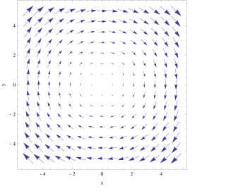
In vector calculus, the curl, also known as rotor, is a vector operator that describes the infinitesimal circulation of a vector field in three-dimensional Euclidean space. The curl at a point in the field is represented by a vector whose length and direction denote the magnitude and axis of the maximum circulation. The curl of a field is formally defined as the circulation density at each point of the field.

Maxwell's equations, or Maxwell–Heaviside equations, are a set of coupled partial differential equations that, together with the Lorentz force law, form the foundation of classical electromagnetism, classical optics, electric and magnetic circuits. The equations provide a mathematical model for electric, optical, and radio technologies, such as power generation, electric motors, wireless communication, lenses, radar, etc. They describe how electric and magnetic fields are generated by charges, currents, and changes of the fields. The equations are named after the physicist and mathematician James Clerk Maxwell, who, in 1861 and 1862, published an early form of the equations that included the Lorentz force law. Maxwell first used the equations to propose that light is an electromagnetic phenomenon. The modern form of the equations in their most common formulation is credited to Oliver Heaviside.
In vector calculus and differential geometry the generalized Stokes theorem, also called the Stokes–Cartan theorem, is a statement about the integration of differential forms on manifolds, which both simplifies and generalizes several theorems from vector calculus. In particular, the fundamental theorem of calculus is the special case where the manifold is a line segment, Green’s theorem and Stokes' theorem are the cases of a surface in or and the divergence theorem is the case of a volume in Hence, the theorem is sometimes referred to as the Fundamental Theorem of Multivariate Calculus.

In mathematics, the orthogonal group in dimension n, denoted O(n), is the group of distance-preserving transformations of a Euclidean space of dimension n that preserve a fixed point, where the group operation is given by composing transformations. The orthogonal group is sometimes called the general orthogonal group, by analogy with the general linear group. Equivalently, it is the group of n × n orthogonal matrices, where the group operation is given by matrix multiplication (an orthogonal matrix is a real matrix whose inverse equals its transpose). The orthogonal group is an algebraic group and a Lie group. It is compact.
In mathematics, especially vector calculus and differential topology, a closed form is a differential form α whose exterior derivative is zero, and an exact form is a differential form, α, that is the exterior derivative of another differential form β. Thus, an exact form is in the image of d, and a closed form is in the kernel of d.
In vector calculus, a vector potential is a vector field whose curl is a given vector field. This is analogous to a scalar potential, which is a scalar field whose gradient is a given vector field.
In vector calculus, a conservative vector field is a vector field that is the gradient of some function. A conservative vector field has the property that its line integral is path independent; the choice of path between two points does not change the value of the line integral. Path independence of the line integral is equivalent to the vector field under the line integral being conservative. A conservative vector field is also irrotational; in three dimensions, this means that it has vanishing curl. An irrotational vector field is necessarily conservative provided that the domain is simply connected.

In mathematical physics, scalar potential, simply stated, describes the situation where the difference in the potential energies of an object in two different positions depends only on the positions, not upon the path taken by the object in traveling from one position to the other. It is a scalar field in three-space: a directionless value (scalar) that depends only on its location. A familiar example is potential energy due to gravity.
In the mathematical field of differential geometry, the exterior covariant derivative is an extension of the notion of exterior derivative to the setting of a differentiable principal bundle or vector bundle with a connection.
In fluid mechanics, the Taylor–Proudman theorem states that when a solid body is moved slowly within a fluid that is steadily rotated with a high angular velocity , the fluid velocity will be uniform along any line parallel to the axis of rotation. must be large compared to the movement of the solid body in order to make the Coriolis force large compared to the acceleration terms.
In algebraic geometry and the theory of complex manifolds, a logarithmic differential form is a differential form with poles of a certain kind. The concept was introduced by Pierre Deligne. In short, logarithmic differentials have the mildest possible singularities needed in order to give information about an open submanifold.
In mathematics, a (real) Monge–Ampère equation is a nonlinear second-order partial differential equation of special kind. A second-order equation for the unknown function u of two variables x,y is of Monge–Ampère type if it is linear in the determinant of the Hessian matrix of u and in the second-order partial derivatives of u. The independent variables (x,y) vary over a given domain D of R2. The term also applies to analogous equations with n independent variables. The most complete results so far have been obtained when the equation is elliptic.
In the differential geometry of surfaces, a Darboux frame is a natural moving frame constructed on a surface. It is the analog of the Frenet–Serret frame as applied to surface geometry. A Darboux frame exists at any non-umbilic point of a surface embedded in Euclidean space. It is named after French mathematician Jean Gaston Darboux.
In continuum mechanics the flow velocity in fluid dynamics, also macroscopic velocity in statistical mechanics, or drift velocity in electromagnetism, is a vector field used to mathematically describe the motion of a continuum. The length of the flow velocity vector is scalar, the flow speed. It is also called velocity field; when evaluated along a line, it is called a velocity profile.
In mathematics, the Riemannian connection on a surface or Riemannian 2-manifold refers to several intrinsic geometric structures discovered by Tullio Levi-Civita, Élie Cartan and Hermann Weyl in the early part of the twentieth century: parallel transport, covariant derivative and connection form. These concepts were put in their current form with principal bundles only in the 1950s. The classical nineteenth century approach to the differential geometry of surfaces, due in large part to Carl Friedrich Gauss, has been reworked in this modern framework, which provides the natural setting for the classical theory of the moving frame as well as the Riemannian geometry of higher-dimensional Riemannian manifolds. This account is intended as an introduction to the theory of connections.
In fluid dynamics, The projection method is an effective means of numerically solving time-dependent incompressible fluid-flow problems. It was originally introduced by Alexandre Chorin in 1967 as an efficient means of solving the incompressible Navier-Stokes equations. The key advantage of the projection method is that the computations of the velocity and the pressure fields are decoupled.
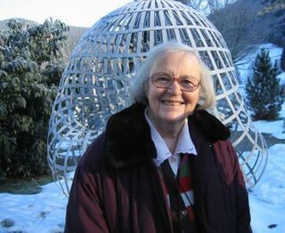
Yvonne Choquet-Bruhat is a French mathematician and physicist. She has made seminal contributions to the study of Einstein's general theory of relativity, by showing that the Einstein equations can be put into the form of an initial value problem which is well-posed. In 2015, her breakthrough paper was listed by the journal Classical and Quantum Gravity as one of thirteen 'milestone' results in the study of general relativity, across the hundred years in which it had been studied.
In vector calculus, a Beltrami vector field, named after Eugenio Beltrami, is a vector field in three dimensions that is parallel to its own curl. That is, F is a Beltrami vector field provided that

Stokes' theorem, also known as the Kelvin–Stokes theorem after Lord Kelvin and George Stokes, the fundamental theorem for curls or simply the curl theorem, is a theorem in vector calculus on . Given a vector field, the theorem relates the integral of the curl of the vector field over some surface, to the line integral of the vector field around the boundary of the surface. The classical theorem of Stokes can be stated in one sentence: The line integral of a vector field over a loop is equal to the surface integral of its curl over the enclosed surface. It is illustrated in the figure, where the direction of positive circulation of the bounding contour ∂Σ, and the direction n of positive flux through the surface Σ, are related by a right-hand-rule. For the right hand the fingers circulate along ∂Σ and the thumb is directed along n.
In fluid dynamics, Lamb surfaces are smooth, connected orientable two-dimensional surfaces, which are simultaneously stream-surfaces and vortex surfaces, named after the physicist Horace Lamb. Lamb surfaces are orthogonal to the Lamb vector everywhere, where and are the vorticity and velocity field, respectively. The necessary and sufficient condition are

