Deconvolution

Last updated August 11, 2023

In mathematics, deconvolution is the operation inverse to convolution. Both operations are used in signal processing and image processing. For example, it may be possible to recover the original signal after a filter (convolution) by using a deconvolution method with a certain degree of accuracy.^[1] Due to the measurement error of the recorded signal or image, it can be demonstrated that the worse the signal-to-noise ratio (SNR), the worse the reversing of a filter will be; hence, inverting a filter is not always a good solution as the error amplifies. Deconvolution offers a solution to this problem.

The foundations for deconvolution and time-series analysis were largely laid by Norbert Wiener of the Massachusetts Institute of Technology in his book Extrapolation, Interpolation, and Smoothing of Stationary Time Series (1949).^[2] The book was based on work Wiener had done during World War II but that had been classified at the time. Some of the early attempts to apply these theories were in the fields of weather forecasting and economics.

Description

In general, the objective of deconvolution is to find the solution f of a convolution equation of the form:

f*g=h\,

Usually, h is some recorded signal, and f is some signal that we wish to recover, but has been convolved with a filter or distortion function g, before we recorded it. Usually, h is a distorted version of f and the shape of f can't be easily recognized by the eye or simpler time-domain operations. The function g represents the impulse response of an instrument or a driving force that was applied to a physical system. If we know g, or at least know the form of g, then we can perform deterministic deconvolution. However, if we do not know g in advance, then we need to estimate it. This can be done using methods of statistical estimation or building the physical principles of the underlying system, such as the electrical circuit equations or diffusion equations.

There are several deconvolution techniques, depending on the choice of the measurement error and deconvolution parameters:

Raw deconvolution

When the measurement error is very low (ideal case), deconvolution collapses into a filter reversing. This kind of deconvolution can be performed in the Laplace domain. By computing the Fourier transform of the recorded signal h and the system response function g, you get H and G, with G as the transfer function. Using to the Convolution theorem,

F=H/G\,

where F is the estimated Fourier transform of f. Finally, the inverse Fourier transform of the function F is taken to find the estimated deconvolved signal f. Note that G is at the denominator and could amplify elements of the error model if present.

Deconvolution with noise

In physical measurements, the situation is usually closer to

(f*g)+\varepsilon =h\,

In this case ε is noise that has entered our recorded signal. If a noisy signal or image is assumed to be noiseless, the statistical estimate of g will be incorrect. In turn, the estimate of ƒ will also be incorrect. The lower the signal-to-noise ratio, the worse the estimate of the deconvolved signal will be. That is the reason why inverse filtering the signal (as in the "raw deconvolution" above) is usually not a good solution. However, if at least some knowledge exists of the type of noise in the data (for example, white noise), the estimate of ƒ can be improved through techniques such as Wiener deconvolution.

Applications

Seismology

The concept of deconvolution had an early application in reflection seismology. In 1950, Enders Robinson was a graduate student at MIT. He worked with others at MIT, such as Norbert Wiener, Norman Levinson, and economist Paul Samuelson, to develop the "convolutional model" of a reflection seismogram. This model assumes that the recorded seismogram s(t) is the convolution of an Earth-reflectivity function e(t) and a seismic wavelet w(t) from a point source, where t represents recording time. Thus, our convolution equation is

s(t)=(e*w)(t).\,

The seismologist is interested in e, which contains information about the Earth's structure. By the convolution theorem, this equation may be Fourier transformed to

S(\omega )=E(\omega )W(\omega )\,

in the frequency domain, where $\omega$ is the frequency variable. By assuming that the reflectivity is white, we can assume that the power spectrum of the reflectivity is constant, and that the power spectrum of the seismogram is the spectrum of the wavelet multiplied by that constant. Thus,

|S(\omega )|\approx k|W(\omega )|.\,

If we assume that the wavelet is minimum phase, we can recover it by calculating the minimum phase equivalent of the power spectrum we just found. The reflectivity may be recovered by designing and applying a Wiener filter that shapes the estimated wavelet to a Dirac delta function (i.e., a spike). The result may be seen as a series of scaled, shifted delta functions (although this is not mathematically rigorous):

e(t)=\sum _{i=1}^{N}r_{i}\delta (t-\tau _{i}),

where N is the number of reflection events, $r_{i}$ are the reflection coefficients, $t-\tau _{i}$ are the reflection times of each event, and $\delta$ is the Dirac delta function.

In practice, since we are dealing with noisy, finite bandwidth, finite length, discretely sampled datasets, the above procedure only yields an approximation of the filter required to deconvolve the data. However, by formulating the problem as the solution of a Toeplitz matrix and using Levinson recursion, we can relatively quickly estimate a filter with the smallest mean squared error possible. We can also do deconvolution directly in the frequency domain and get similar results. The technique is closely related to linear prediction.

Optics and other imaging

In optics and imaging, the term "deconvolution" is specifically used to refer to the process of reversing the optical distortion that takes place in an optical microscope, electron microscope, telescope, or other imaging instrument, thus creating clearer images. It is usually done in the digital domain by a software algorithm, as part of a suite of microscope image processing techniques. Deconvolution is also practical to sharpen images that suffer from fast motion or jiggles during capturing. Early Hubble Space Telescope images were distorted by a flawed mirror and were sharpened by deconvolution.

The usual method is to assume that the optical path through the instrument is optically perfect, convolved with a point spread function (PSF), that is, a mathematical function that describes the distortion in terms of the pathway a theoretical point source of light (or other waves) takes through the instrument.^[3] Usually, such a point source contributes a small area of fuzziness to the final image. If this function can be determined, it is then a matter of computing its inverse or complementary function, and convolving the acquired image with that. The result is the original, undistorted image.

In practice, finding the true PSF is impossible, and usually an approximation of it is used, theoretically calculated^[4] or based on some experimental estimation by using known probes. Real optics may also have different PSFs at different focal and spatial locations, and the PSF may be non-linear. The accuracy of the approximation of the PSF will dictate the final result. Different algorithms can be employed to give better results, at the price of being more computationally intensive. Since the original convolution discards data, some algorithms use additional data acquired at nearby focal points to make up some of the lost information. Regularization in iterative algorithms (as in expectation-maximization algorithms) can be applied to avoid unrealistic solutions.

When the PSF is unknown, it may be possible to deduce it by systematically trying different possible PSFs and assessing whether the image has improved. This procedure is called blind deconvolution .^[3] Blind deconvolution is a well-established image restoration technique in astronomy, where the point nature of the objects photographed exposes the PSF thus making it more feasible. It is also used in fluorescence microscopy for image restoration, and in fluorescence spectral imaging for spectral separation of multiple unknown fluorophores. The most common iterative algorithm for the purpose is the Richardson–Lucy deconvolution algorithm; the Wiener deconvolution (and approximations) are the most common non-iterative algorithms.

For some specific imaging systems such as laser pulsed terahertz systems, PSF can be modeled mathematically.^[6] As a result, as shown in the figure, deconvolution of the modeled PSF and the terahertz image can give a higher resolution representation of the terahertz image.

Radio astronomy

When performing image synthesis in radio interferometry, a specific kind of radio astronomy, one step consists of deconvolving the produced image with the "dirty beam", which is a different name for the point spread function. A commonly used method is the CLEAN algorithm.

Biology, physiology and medical devices

Typical use of deconvolution is in tracer kinetics. For example, when measuring a hormone concentration in the blood, its secretion rate can be estimated by deconvolution. Another example is the estimation of the blood glucose concentration from the measured interstitial glucose, which is a distorted version in time and amplitude of the real blood glucose. ^[7]

Absorption spectra

Deconvolution has been applied extensively to absorption spectra.^[8] The Van Cittert algorithm (article in German) may be used.^[9]

Fourier transform aspects

Deconvolution maps to division in the Fourier co-domain. This allows deconvolution to be easily applied with experimental data that are subject to a Fourier transform. An example is NMR spectroscopy where the data are recorded in the time domain, but analyzed in the frequency domain. Division of the time-domain data by an exponential function has the effect of reducing the width of Lorentzian lines in the frequency domain.

Related Research Articles

In mathematics, the discrete Fourier transform (DFT) converts a finite sequence of equally-spaced samples of a function into a same-length sequence of equally-spaced samples of the discrete-time Fourier transform (DTFT), which is a complex-valued function of frequency. The interval at which the DTFT is sampled is the reciprocal of the duration of the input sequence. An inverse DFT (IDFT) is a Fourier series, using the DTFT samples as coefficients of complex sinusoids at the corresponding DTFT frequencies. It has the same sample-values as the original input sequence. The DFT is therefore said to be a frequency domain representation of the original input sequence. If the original sequence spans all the non-zero values of a function, its DTFT is continuous, and the DFT provides discrete samples of one cycle. If the original sequence is one cycle of a periodic function, the DFT provides all the non-zero values of one DTFT cycle.

In engineering, a transfer function of a system, sub-system, or component is a mathematical function that models the system's output for each possible input. They are widely used in electronic engineering tools like circuit simulators and control systems. In some simple cases, this function can be represented as two-dimensional graph of an independent scalar input versus the dependent scalar output, called a transfer curve or characteristic curve. Transfer functions for components are used to design and analyze systems assembled from components, particularly using the block diagram technique, in electronics and control theory.

A wavelet is a wave-like oscillation with an amplitude that begins at zero, increases or decreases, and then returns to zero one or more times. Wavelets are termed a "brief oscillation". A taxonomy of wavelets has been established, based on the number and direction of its pulses. Wavelets are imbued with specific properties that make them useful for signal processing.

<span class="mw-page-title-main">Fourier transform</span> Mathematical transform that expresses a function of time as a function of frequency

In physics and mathematics, the Fourier transform (FT) is a transform that converts a function into a form that describes the frequencies present in the original function. The output of the transform is a complex-valued function of frequency. The term Fourier transform refers to both this complex-valued function and the mathematical operation. When a distinction needs to be made the Fourier transform is sometimes called the frequency domain representation of the original function. The Fourier transform is analogous to decomposing the sound of a musical chord into terms of the intensity of its constituent pitches.

Fourier optics is the study of classical optics using Fourier transforms (FTs), in which the waveform being considered is regarded as made up of a combination, or superposition, of plane waves. It has some parallels to the Huygens–Fresnel principle, in which the wavefront is regarded as being made up of a combination of spherical wavefronts whose sum is the wavefront being studied. A key difference is that Fourier optics considers the plane waves to be natural modes of the propagation medium, as opposed to Huygens–Fresnel, where the spherical waves originate in the physical medium.

In mathematics, the Gibbs phenomenon is the oscillatory behavior of the Fourier series of a piecewise continuously differentiable periodic function around a jump discontinuity. The $th partial Fourier series of the function produces large peaks around the jump which overshoot and undershoot the function values. As more sinusoids are used, this approximation error approaches a limit of about 9% of the jump, though the infinite Fourier series sum does eventually converge almost everywhere except points of discontinuity.$

Analog signal processing is a type of signal processing conducted on continuous analog signals by some analog means. "Analog" indicates something that is mathematically represented as a set of continuous values. This differs from "digital" which uses a series of discrete quantities to represent signal. Analog values are typically represented as a voltage, electric current, or electric charge around components in the electronic devices. An error or noise affecting such physical quantities will result in a corresponding error in the signals represented by such physical quantities.

In signal processing, a finite impulse response (FIR) filter is a filter whose impulse response is of finite duration, because it settles to zero in finite time. This is in contrast to infinite impulse response (IIR) filters, which may have internal feedback and may continue to respond indefinitely.

In mathematics, the continuous wavelet transform (CWT) is a formal tool that provides an overcomplete representation of a signal by letting the translation and scale parameter of the wavelets vary continuously.

<span class="mw-page-title-main">Point spread function</span> Response in an optical imaging system

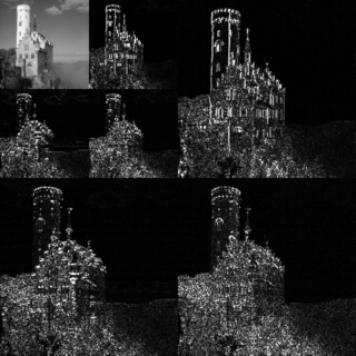
The point spread function (PSF) describes the response of a focused optical imaging system to a point source or point object. A more general term for the PSF is the system's impulse response; the PSF is the impulse response or impulse response function (IRF) of a focused optical imaging system. The PSF in many contexts can be thought of as the extended blob in an image that represents a single point object, that is considered as a spatial impulse. In functional terms, it is the spatial domain version of the optical transfer function (OTF) of an imaging system. It is a useful concept in Fourier optics, astronomical imaging, medical imaging, electron microscopy and other imaging techniques such as 3D microscopy and fluorescence microscopy.

In mathematics, in the area of harmonic analysis, the fractional Fourier transform (FRFT) is a family of linear transformations generalizing the Fourier transform. It can be thought of as the Fourier transform to the n-th power, where n need not be an integer — thus, it can transform a function to any intermediate domain between time and frequency. Its applications range from filter design and signal analysis to phase retrieval and pattern recognition.

In electrical engineering and applied mathematics, blind deconvolution is deconvolution without explicit knowledge of the impulse response function used in the convolution. This is usually achieved by making appropriate assumptions of the input to estimate the impulse response by analyzing the output. Blind deconvolution is not solvable without making assumptions on input and impulse response. Most of the algorithms to solve this problem are based on assumption that both input and impulse response live in respective known subspaces. However, blind deconvolution remains a very challenging non-convex optimization problem even with this assumption.

In signal processing, a causal filter is a linear and time-invariant causal system. The word causal indicates that the filter output depends only on past and present inputs. A filter whose output also depends on future inputs is non-causal, whereas a filter whose output depends only on future inputs is anti-causal. Systems that are realizable must be causal because such systems cannot act on a future input. In effect that means the output sample that best represents the input at time $comes out slightly later. A common design practice for digital filters is to create a realizable filter by shortening and/or time-shifting a non-causal impulse response. If shortening is necessary, it is often accomplished as the product of the impulse-response with a window function.$

In mathematics, a wavelet series is a representation of a square-integrable function by a certain orthonormal series generated by a wavelet. This article provides a formal, mathematical definition of an orthonormal wavelet and of the integral wavelet transform.

In mathematics, Wiener deconvolution is an application of the Wiener filter to the noise problems inherent in deconvolution. It works in the frequency domain, attempting to minimize the impact of deconvolved noise at frequencies which have a poor signal-to-noise ratio.

Phase stretch transform (PST) is a computational approach to signal and image processing. One of its utilities is for feature detection and classification. PST is related to time stretch dispersive Fourier transform. It transforms the image by emulating propagation through a diffractive medium with engineered 3D dispersive property. The operation relies on symmetry of the dispersion profile and can be understood in terms of dispersive eigenfunctions or stretch modes. PST performs similar functionality as phase-contrast microscopy, but on digital images. PST can be applied to digital images and temporal data. It is a physics-based feature engineering algorithm.

In signal processing, nonlinear multidimensional signal processing (NMSP) covers all signal processing using nonlinear multidimensional signals and systems. Nonlinear multidimensional signal processing is a subset of signal processing (multidimensional signal processing). Nonlinear multi-dimensional systems can be used in a broad range such as imaging, teletraffic, communications, hydrology, geology, and economics. Nonlinear systems cannot be treated as linear systems, using Fourier transformation and wavelet analysis. Nonlinear systems will have chaotic behavior, limit cycle, steady state, bifurcation, multi-stability and so on. Nonlinear systems do not have a canonical representation, like impulse response for linear systems. But there are some efforts to characterize nonlinear systems, such as Volterra and Wiener series using polynomial integrals as the use of those methods naturally extend the signal into multi-dimensions. Another example is the Empirical mode decomposition method using Hilbert transform instead of Fourier Transform for nonlinear multi-dimensional systems. This method is an empirical method and can be directly applied to data sets. Multi-dimensional nonlinear filters (MDNF) are also an important part of NMSP, MDNF are mainly used to filter noise in real data. There are nonlinear-type hybrid filters used in color image processing, nonlinear edge-preserving filters use in magnetic resonance image restoration. Those filters use both temporal and spatial information and combine the maximum likelihood estimate with the spatial smoothing algorithm.

Multidimensional seismic data processing forms a major component of seismic profiling, a technique used in geophysical exploration. The technique itself has various applications, including mapping ocean floors, determining the structure of sediments, mapping subsurface currents and hydrocarbon exploration. Since geophysical data obtained in such techniques is a function of both space and time, multidimensional signal processing techniques may be better suited for processing such data.

In multidimensional signal processing, Multidimensional signal restoration refers to the problem of estimating the original input signal from observations of the distorted or noise contaminated version of the original signal using some prior information about the input signal and /or the distortion process. Multidimensional signal processing systems such as audio, image and video processing systems often receive as input, signals that undergo distortions like blurring, band-limiting etc. during signal acquisition or transmission and it may be vital to recover the original signal for further filtering. Multidimensional signal restoration is an inverse problem, where only the distorted signal is observed and some information about the distortion process and/or input signal properties is known. A general class of iterative methods have been developed for the multidimensional restoration problem with successful applications to multidimensional deconvolution, signal extrapolation and denoising.

Lightfieldmicroscopy (LFM) is a scanning-free 3-dimensional (3D) microscopic imaging method based on the theory of light field. This technique allows sub-second (~10 Hz) large volumetric imaging with ~1 μm spatial resolution in the condition of weak scattering and semi-transparence, which has never been achieved by other methods. Just as in traditional light field rendering, there are two steps for LFM imaging: light field capture and processing. In most setups, a microlens array is used to capture the light field. As for processing, it can be based on two kinds of representations of light propagation: the ray optics picture and the wave optics picture. The Stanford University Computer Graphics Laboratory published their first prototype LFM in 2006 and has been working on the cutting edge since then.

References

↑ O'Haver, T. "Intro to Signal Processing - Deconvolution". University of Maryland at College Park. Retrieved 2007-08-15.
↑ Wiener, N. (1964). Extrapolation, Interpolation, and Smoothing of Stationary Time Series. Cambridge, Mass: MIT Press. ISBN 0-262-73005-7.
1 2 Cheng, P. C. (2006). "The Contrast Formation in Optical Microscopy". In Pawley, J. B. (ed.). Handbook of Biological Confocal Microscopy (3rd ed.). Berlin: Springer. pp. 189–90. ISBN 0-387-25921-X.
↑ Nasse, M. J.; Woehl, J. C. (2010). "Realistic modeling of the illumination point spread function in confocal scanning optical microscopy". Journal of the Optical Society of America A. 27 (2): 295–302. Bibcode:2010JOSAA..27..295N. doi:10.1364/JOSAA.27.000295. PMID 20126241.
↑ Ahi, Kiarash; Anwar, Mehdi (May 26, 2016). Anwar, Mehdi F; Crowe, Thomas W; Manzur, Tariq (eds.). "Developing terahertz imaging equation and enhancement of the resolution of terahertz images using deconvolution". Proc. SPIE 9856, Terahertz Physics, Devices, and Systems X: Advanced Applications in Industry and Defense, 98560N. Terahertz Physics, Devices, and Systems X: Advanced Applications in Industry and Defense. 9856: 98560N. Bibcode:2016SPIE.9856E..0NA. doi:10.1117/12.2228680. S2CID 114994724.
↑ Sung, Shijun (2013). Terahertz Imaging and Remote Sensing Design for Applications in Medical Imaging. UCLA Electronic Theses and Dissertations.
↑ Sparacino, Giovanni; Cobelli, Claudio (1996). "Reconstruction of insulin secretion rate by deconvolution: domain of validity of a monoexponential C-peptide impulse response model". Techno Health Care. 4 (1): 87–9511. doi:10.3233/THC-1996-4110. PMID 8773311.
↑ Blass, W. E.; Halsey, G. W. (1981). Deconvolution of Absorption Spectra . Academic Press. ISBN 0121046508.
↑ Wu, Chengqi; Aissaoui, Idriss; Jacquey, Serge (1994). "Algebraic analysis of the Van Cittert iterative method of deconvolution with a general relaxation factor". J. Opt. Soc. Am. A. 11 (11): 2804–2808. Bibcode:1994JOSAA..11.2804X. doi:10.1364/JOSAA.11.002804.

This page is based on this Wikipedia article
Text is available under the CC BY-SA 4.0 license; additional terms may apply.
Images, videos and audio are available under their respective licenses.

[1] O'Haver, T. "Intro to Signal Processing - Deconvolution". University of Maryland at College Park. Retrieved 2007-08-15.

[2] Wiener, N. (1964). Extrapolation, Interpolation, and Smoothing of Stationary Time Series. Cambridge, Mass: MIT Press. ISBN 0-262-73005-7.

[Pawley_2006-3] 1 2 Cheng, P. C. (2006). "The Contrast Formation in Optical Microscopy". In Pawley, J. B. (ed.). Handbook of Biological Confocal Microscopy (3rd ed.). Berlin: Springer. pp. 189–90. ISBN 0-387-25921-X.

[4] Nasse, M. J.; Woehl, J. C. (2010). "Realistic modeling of the illumination point spread function in confocal scanning optical microscopy". Journal of the Optical Society of America A. 27 (2): 295–302. Bibcode:2010JOSAA..27..295N. doi:10.1364/JOSAA.27.000295. PMID 20126241.

[5] Ahi, Kiarash; Anwar, Mehdi (May 26, 2016). Anwar, Mehdi F; Crowe, Thomas W; Manzur, Tariq (eds.). "Developing terahertz imaging equation and enhancement of the resolution of terahertz images using deconvolution". Proc. SPIE 9856, Terahertz Physics, Devices, and Systems X: Advanced Applications in Industry and Defense, 98560N. Terahertz Physics, Devices, and Systems X: Advanced Applications in Industry and Defense. 9856: 98560N. Bibcode:2016SPIE.9856E..0NA. doi:10.1117/12.2228680. S2CID 114994724.

[6] Sung, Shijun (2013). Terahertz Imaging and Remote Sensing Design for Applications in Medical Imaging. UCLA Electronic Theses and Dissertations.

[7] Sparacino, Giovanni; Cobelli, Claudio (1996). "Reconstruction of insulin secretion rate by deconvolution: domain of validity of a monoexponential C-peptide impulse response model". Techno Health Care. 4 (1): 87–9511. doi:10.3233/THC-1996-4110. PMID 8773311.

[8] Blass, W. E.; Halsey, G. W. (1981). Deconvolution of Absorption Spectra . Academic Press. ISBN 0121046508.

[9] Wu, Chengqi; Aissaoui, Idriss; Jacquey, Serge (1994). "Algebraic analysis of the Van Cittert iterative method of deconvolution with a general relaxation factor". J. Opt. Soc. Am. A. 11 (11): 2804–2808. Bibcode:1994JOSAA..11.2804X. doi:10.1364/JOSAA.11.002804.

[1]

[2]

[3]

[4]

[6]

[7]

[8]

[9]