Hough transform

Last updated

The Hough transform is a feature extraction technique used in image analysis, computer vision, pattern recognition, and digital image processing. [1] [2] The purpose of the technique is to find imperfect instances of objects within a certain class of shapes by a voting procedure. This voting procedure is carried out in a parameter space, from which object candidates are obtained as local maxima in a so-called accumulator space that is explicitly constructed by the algorithm for computing the Hough transform.

Contents

The classical Hough transform was concerned with the identification of lines in the image, but later the Hough transform has been extended to identifying positions of arbitrary shapes, most commonly circles or ellipses. The Hough transform as it is universally used today was invented by Richard Duda and Peter Hart in 1972, who called it a "generalized Hough transform" [3] after the related 1962 patent of Paul Hough. [4] [5] The transform was popularized in the computer vision community by Dana H. Ballard through a 1981 journal article titled "Generalizing the Hough transform to detect arbitrary shapes".

History

It was initially invented for machine analysis of bubble chamber photographs (Hough, 1959).

The Hough transform was patented as U.S. patent 3,069,654 in 1962 and assigned to the U.S. Atomic Energy Commission with the name "Method and Means for Recognizing Complex Patterns". This patent uses a slope-intercept parametrization for straight lines, which awkwardly leads to an unbounded transform space since the slope can go to infinity.

The rho-theta parametrization universally used today was first described in

Duda, R.O.; Hart, P. E. (January 1972). "Use of the Hough Transformation to Detect Lines and Curves in Pictures". Comm. ACM. 15: 11–15. doi: 10.1145/361237.361242 . S2CID   1105637.

although it was already standard for the Radon transform since at least the 1930s.

O'Gorman and Clowes' variation is described in

O'Gorman, Frank; Clowes, MB (1976). "Finding Picture Edges Through Collinearity of Feature Points". IEEE Trans. Comput. 25 (4): 449–456. doi:10.1109/TC.1976.1674627. S2CID   10851078.

The story of how the modern form of the Hough transform was invented is given in

Hart, P. E. (November 2009). "How the Hough Transform was Invented" (PDF). IEEE Signal Processing Magazine. 26 (6): 18–22. doi:10.1109/msp.2009.934181. S2CID   16245096. Archived from the original (PDF) on 2018-05-16.

Theory

In automated analysis of digital images, a subproblem often arises of detecting simple shapes, such as straight lines, circles or ellipses. In many cases an edge detector can be used as a pre-processing stage to obtain image points or image pixels that are on the desired curve in the image space. Due to imperfections in either the image data or the edge detector, however, there may be missing points or pixels on the desired curves as well as spatial deviations between the ideal line/circle/ellipse and the noisy edge points as they are obtained from the edge detector. For these reasons, it is often non-trivial to group the extracted edge features to an appropriate set of lines, circles or ellipses. The purpose of the Hough transform is to address this problem by making it possible to perform groupings of edge points into object candidates by performing an explicit voting procedure over a set of parameterized image objects (Shapiro and Stockman, 304).

Detecting lines

The simplest case of Hough transform is detecting straight lines. In general, the straight line y = mx + b can be represented as a point (b, m) in the parameter space. However, vertical lines pose a problem. They would give rise to unbounded values of the slope parameter m. Thus, for computational reasons, Duda and Hart [6] proposed the use of the Hesse normal form

where is the distance from the origin to the closest point on the straight line, and is the angle between the axis and the line connecting the origin with that closest point.

The intuition for this form, similarly to the plane equation, is that every vector on the line must be perpendicular (orthogonal) to the straight line of length that comes from the origin. It can be seen that the intersection point of the function line and the perpendicular line that comes from the origin is at . So, for any point on the line, the vector must be orthogonal to the vector . Therefore, we get that for any point on the function line, the equation must be satisfied. Therefore, . Since and , we get . Since , we get the final form of .

R theta line.GIF

It is therefore possible to associate with each line of the image a pair . The plane is sometimes referred to as Hough space for the set of straight lines in two dimensions. This representation makes the Hough transform conceptually very close to the two-dimensional Radon transform. In fact, the Hough transform is mathematically equivalent to the Radon transform, but the two transformations have different computational interpretations traditionally associated with them. [7]

Given a single point in the plane, the set of all straight lines going through that point corresponds to a sinusoidal curve in the (r, θ) plane, which is unique to that point. A set of two or more points that form a straight line will produce sinusoids crossing at the (r, θ) for that line. Thus, the problem of detecting collinear points can be converted to the problem of finding concurrent curves.

Probabilistic interpretation

Given a shape parametrized by , taking values in the set called the shape space, one can interpret the Hough transform as the inverse transform of a probability distribution on the image space to the shape space , and interpret shape detection as maximum likelihood estimation.

Explicitly, the Hough transform performs an approximate naive Bayes inference. We start with a uniform prior on the shape space. We consider only the positive evidence, and ignore all negative evidence, so that we can detect partially occluded shapes.

We add up the log-likelihood in the shape space up to an additive constant. The assumption of naive Bayes means that all pixels in the image space provide independent evidence, so that their likelihoods multiply, that is, their log-likelihoods add. The freedom in additive constant allows us to perform no operation on the "background pixels" in shape space.

Finally, we perform maximum likelihood estimation by picking out the peaks in the log-likelihood on the shape space. [8]

Derivations

Implementation

The linear Hough transform algorithm estimates the two parameters that define a straight line. The transform space has two dimensions, and every point in the transform space is used as an accumulator to detect or identify a line described by . Every point in the detected edges in the image contributes to the accumulators.

The dimension of the accumulator equals the number of unknown parameters, i.e., two, considering quantized values of and in the pair . For each pixel at and its neighborhood, the Hough transform algorithm determines whether there is enough evidence of a straight line at that pixel. If so, it will calculate the parameters of that line, then look for the accumulator's bin that the parameters fall into, and increment the value of that bin.

By finding the bins with the highest values, typically by looking for local maxima in the accumulator space, the most likely lines can be extracted, and their (approximate) geometric definitions read off (Shapiro and Stockman, 304). The simplest way of finding these peaks is by applying some form of threshold, but other techniques may yield better results in different circumstances – determining which lines are found, as well as how many. Since the lines returned do not contain any length information, it is often necessary, in the next step, to find which parts of the image match up with which lines. Moreover, due to imperfection errors in the edge-detection step, there will usually be errors in the accumulator space, which may make it non-trivial to find the appropriate peaks, and thus the appropriate lines.

The final result of the linear Hough transform is a two-dimensional array (matrix) similar to the accumulator—one dimension of this matrix is the quantized angle , and the other dimension is the quantized distance . Each element of the matrix has a value equal to the sum of the points or pixels that are positioned on the line represented by quantized parameters . So the element with the highest value indicates the straight line that is most represented in the input image. [9]

Examples

Example 1

Consider three data points, shown here as black dots.

Example 1 Hough transform diagram.svg
Example 1

From the calculations, it can be seen that in either case the support line at 60° has a similar length. Hence, it is understood that the corresponding lines (the blue ones in the above picture) are very similar. One can thus assume that all points lie close to the blue line.

Example 2

The following is a different example showing the results of a Hough transform on a raster image containing two thick lines.

Hough-example-result-en.png

The results of this transform were stored in a matrix. Cell value represents the number of curves through any point. Higher cell values are rendered brighter. The two distinctly bright spots are the Hough parameters of the two lines. From these spots' positions, angle and distance from image center of the two lines in the input image can be determined.

Variations and extensions

Using the gradient direction to reduce the number of votes

An improvement suggested by O'Gorman and Clowes can be used to detect lines if one takes into account that the local gradient of the image intensity will necessarily be orthogonal to the edge. Since edge detection generally involves computing the intensity gradient magnitude, the gradient direction is often found as a side effect. If a given point of coordinates (x,y) happens to indeed be on a line, then the local direction of the gradient gives the θ parameter corresponding to said line, and the r parameter is then immediately obtained. (Shapiro and Stockman, 305) The gradient direction can be estimated to within 20°, which shortens the sinusoid trace from the full 180° to roughly 45°. This reduces the computation time and has the interesting effect of reducing the number of useless votes, thus enhancing the visibility of the spikes corresponding to real lines in the image.

Kernel-based Hough transform (KHT)

Fernandes and Oliveira [10] suggested an improved voting scheme for the Hough transform that allows a software implementation to achieve real-time performance even on relatively large images (e.g., 1280×960). The Kernel-based Hough transform uses the same parameterization proposed by Duda and Hart but operates on clusters of approximately collinear pixels. For each cluster, votes are cast using an oriented elliptical-Gaussian kernel that models the uncertainty associated with the best-fitting line with respect to the corresponding cluster. The approach not only significantly improves the performance of the voting scheme, but also produces a much cleaner accumulator and makes the transform more robust to the detection of spurious lines.

3-D kernel-based Hough transform for plane detection (3DKHT)

Limberger and Oliveira [11] suggested a deterministic technique for plane detection in unorganized point clouds whose cost is in the number of samples, achieving real-time performance for relatively large datasets (up to points on a 3.4 GHz CPU). It is based on a fast Hough-transform voting strategy for planar regions, inspired by the Kernel-based Hough transform (KHT). This 3D kernel-based Hough transform (3DKHT) uses a fast and robust algorithm to segment clusters of approximately co-planar samples, and casts votes for individual clusters (instead of for individual samples) on a () spherical accumulator using a trivariate Gaussian kernel. The approach is several orders of magnitude faster than existing (non-deterministic) techniques for plane detection in point clouds, such as RHT and RANSAC, and scales better with the size of the datasets. It can be used with any application that requires fast detection of planar features on large datasets.

Hough transform of curves, and its generalization for analytical and non-analytical shapes

Although the version of the transform described above applies only to finding straight lines, a similar transform can be used for finding any shape which can be represented by a set of parameters. A circle, for instance, can be transformed into a set of three parameters, representing its center and radius, so that the Hough space becomes three dimensional. Arbitrary ellipses and curves can also be found this way, as can any shape easily expressed as a set of parameters.

The generalization of the Hough transform for detecting analytical shapes in spaces having any dimensionality was proposed by Fernandes and Oliveira. [12] In contrast to other Hough transform-based approaches for analytical shapes, Fernandes' technique does not depend on the shape one wants to detect nor on the input data type. The detection can be driven to a type of analytical shape by changing the assumed model of geometry where data have been encoded (e.g., euclidean space, projective space, conformal geometry, and so on), while the proposed formulation remains unchanged. Also, it guarantees that the intended shapes are represented with the smallest possible number of parameters, and it allows the concurrent detection of different kinds of shapes that best fit an input set of entries with different dimensionalities and different geometric definitions (e.g., the concurrent detection of planes and spheres that best fit a set of points, straight lines and circles).

For more complicated shapes in the plane (i.e., shapes that cannot be represented analytically in some 2D space), the Generalised Hough transform [13] is used, which allows a feature to vote for a particular position, orientation and/or scaling of the shape using a predefined look-up table.The Hough transform accumulates contributions from all pixels in the detected edge.

Circle detection process

Altering the algorithm to detect circular shapes instead of lines is relatively straightforward.

If we do not know the radius of the circle we are trying to locate beforehand, we can use a three-dimensional accumulator space to search for circles with an arbitrary radius. Naturally, this is more computationally expensive.

This method can also detect circles that are partially outside of the accumulator space, as long as enough of the circle's area is still present within it.

Detection of 3D objects (planes and cylinders)

Hough transform can also be used for the detection of 3D objects in range data or 3D point clouds. The extension of classical Hough transform for plane detection is quite straightforward. A plane is represented by its explicit equation for which we can use a 3D Hough space corresponding to , and . This extension suffers from the same problems as its 2D counterpart i.e., near horizontal planes can be reliably detected, while the performance deteriorates as planar direction becomes vertical (big values of and amplify the noise in the data). This formulation of the plane has been used for the detection of planes in the point clouds acquired from airborne laser scanning [14] and works very well because in that domain all planes are nearly horizontal.

For generalized plane detection using Hough transform, the plane can be parametrized by its normal vector (using spherical coordinates) and its distance from the origin resulting in a three dimensional Hough space. This results in each point in the input data voting for a sinusoidal surface in the Hough space. The intersection of these sinusoidal surfaces indicates presence of a plane. [15] A more general approach for more than 3 dimensions requires search heuristics to remain feasible. [16]

Hough transform has also been used to find cylindrical objects in point clouds using a two step approach. The first step finds the orientation of the cylinder and the second step finds the position and radius. [17]

Using weighted features

One common variation detail. That is, finding the bins with the highest count in one stage can be used to constrain the range of values searched in the next.

Carefully chosen parameter space

A high-dimensional parameter space for the Hough transform is not only slow, but if implemented without forethought can easily overrun the available memory. Even if the programming environment allows the allocation of an array larger than the available memory space through virtual memory, the number of page swaps required for this will be very demanding because the accumulator array is used in a randomly accessed fashion, rarely stopping in contiguous memory as it skips from index to index.

Consider the task of finding ellipses in an 800x600 image. Assuming that the radii of the ellipses are oriented along principal axes, the parameter space is four-dimensional. (x, y) defines the center of the ellipse, and a and b denote the two radii. Allowing the center to be anywhere in the image, adds the constraint 0<x<800 and 0<y<600. If the radii are given the same values as constraints, what is left is a sparsely filled accumulator array of more than 230 billion values.

A program thus conceived is unlikely to be allowed to allocate sufficient memory. This doesn't mean that the problem can't be solved, but only that new ways to constrain the size of the accumulator array are to be found, which makes it feasible. For instance:

  1. If it is reasonable to assume that the ellipses are each contained entirely within the image, the range of the radii can be reduced. The largest the radii can be is if the center of the ellipse is in the center of the image, allowing the edges of the ellipse to stretch to the edges. In this extreme case, the radii can only each be half the magnitude of the image size oriented in the same direction. Reducing the range of a and b in this fashion reduces the accumulator array to 57 billion values.
  2. Trade accuracy for space in the estimation of the center: If the center is predicted to be off by 3 on both the x and y axis this reduces the size of the accumulator array to about 6 billion values.
  3. Trade accuracy for space in the estimation of the radii: If the radii are estimated to each be off by 5 further reduction of the size of the accumulator array occurs, by about 256 million values.
  4. Crop the image to areas of interest. This is image dependent, and therefore unpredictable, but imagine a case where all of the edges of interest in an image are in the upper left quadrant of that image. The accumulator array can be reduced even further in this case by constraining all 4 parameters by a factor of 2, for a total reduction factor of 16.

By applying just the first three of these constraints to the example stated about, the size of the accumulator array is reduced by almost a factor of 1000, bringing it down to a size that is much more likely to fit within a modern computer's memory.

Efficient ellipse detection algorithm

Yonghong Xie and Qiang Ji give an efficient way of implementing the Hough transform for ellipse detection by overcoming the memory issues. [18] As discussed in the algorithm (on page 2 of the paper), this approach uses only a one-dimensional accumulator (for the minor axis) in order to detect ellipses in the image. The complexity is O(N3) in the number of non-zero points in the image.

Limitations

The Hough transform is only efficient if a high number of votes fall in the right bin, so that the bin can be easily detected amid the background noise. This means that the bin must not be too small, or else some votes will fall in the neighboring bins, thus reducing the visibility of the main bin. [19]

Also, when the number of parameters is large (that is, when we are using the Hough transform with typically more than three parameters), the average number of votes cast in a single bin is very low, and those bins corresponding to a real figure in the image do not necessarily appear to have a much higher number of votes than their neighbors. The complexity increases at a rate of with each additional parameter, where is the size of the image space and is the number of parameters. (Shapiro and Stockman, 310) Thus, the Hough transform must be used with great care to detect anything other than lines or circles.

Finally, much of the efficiency of the Hough transform is dependent on the quality of the input data: the edges must be detected well for the Hough transform to be efficient. Use of the Hough transform on noisy images is a very delicate matter and generally, a denoising stage must be used before. In the case where the image is corrupted by speckle, as is the case in radar images, the Radon transform is sometimes preferred to detect lines, because it attenuates the noise through summation.

See also

Related Research Articles

<span class="mw-page-title-main">Ellipse</span> Plane curve: conic section

In mathematics, an ellipse is a plane curve surrounding two focal points, such that for all points on the curve, the sum of the two distances to the focal points is a constant. It generalizes a circle, which is the special type of ellipse in which the two focal points are the same. The elongation of an ellipse is measured by its eccentricity , a number ranging from to .

In mathematics, an equation is a mathematical formula that expresses the equality of two expressions, by connecting them with the equals sign =. The word equation and its cognates in other languages may have subtly different meanings; for example, in French an équation is defined as containing one or more variables, while in English, any well-formed formula consisting of two expressions related with an equals sign is an equation.

<span class="mw-page-title-main">Sphere</span> Set of points equidistant from a center

A sphere is a geometrical object that is a three-dimensional analogue to a two-dimensional circle. Formally, a sphere is the set of points that are all at the same distance r from a given point in three-dimensional space. That given point is the center of the sphere, and r is the sphere's radius. The earliest known mentions of spheres appear in the work of the ancient Greek mathematicians.

In electrodynamics, elliptical polarization is the polarization of electromagnetic radiation such that the tip of the electric field vector describes an ellipse in any fixed plane intersecting, and normal to, the direction of propagation. An elliptically polarized wave may be resolved into two linearly polarized waves in phase quadrature, with their polarization planes at right angles to each other. Since the electric field can rotate clockwise or counterclockwise as it propagates, elliptically polarized waves exhibit chirality.

<span class="mw-page-title-main">Great circle</span> Spherical geometry analog of a straight line

In mathematics, a great circle or orthodrome is the circular intersection of a sphere and a plane passing through the sphere's center point.

<span class="mw-page-title-main">Ellipsoid</span> Quadric surface that looks like a deformed sphere

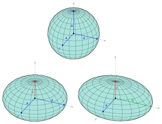
An ellipsoid is a surface that can be obtained from a sphere by deforming it by means of directional scalings, or more generally, of an affine transformation.

<span class="mw-page-title-main">3D projection</span> Design technique

A 3D projection is a design technique used to display a three-dimensional (3D) object on a two-dimensional (2D) surface. These projections rely on visual perspective and aspect analysis to project a complex object for viewing capability on a simpler plane.

<span class="mw-page-title-main">Parametric equation</span> Representation of a curve by a function of a parameter

In mathematics, a parametric equation defines a group of quantities as functions of one or more independent variables called parameters. Parametric equations are commonly used to express the coordinates of the points that make up a geometric object such as a curve or surface, called a parametric curve and parametric surface, respectively. In such cases, the equations are collectively called a parametric representation, or parametric system, or parameterization of the object.

<span class="mw-page-title-main">Cone</span> Geometric shape

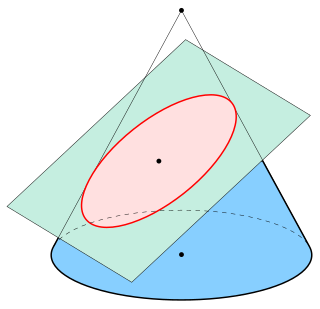
A cone is a three-dimensional geometric shape that tapers smoothly from a flat base to a point called the apex or vertex.

<span class="mw-page-title-main">Cissoid</span> Plane curve constructed from two other curves and a fixed point

In geometry, a cissoid is a plane curve generated from two given curves C1, C2 and a point O. Let L be a variable line passing through O and intersecting C1 at P1 and C2 at P2. Let P be the point on L so that Then the locus of such points P is defined to be the cissoid of the curves C1, C2 relative to O.

<span class="mw-page-title-main">Mollweide projection</span> Pseudocylindrical equal-area map projection

The Mollweide projection is an equal-area, pseudocylindrical map projection generally used for maps of the world or celestial sphere. It is also known as the Babinet projection, homalographic projection, homolographic projection, and elliptical projection. The projection trades accuracy of angle and shape for accuracy of proportions in area, and as such is used where that property is needed, such as maps depicting global distributions.

<span class="mw-page-title-main">Stokes parameters</span> Set of values that describe the polarization state of electromagnetic radiation

The Stokes parameters are a set of values that describe the polarization state of electromagnetic radiation. They were defined by George Gabriel Stokes in 1852, as a mathematically convenient alternative to the more common description of incoherent or partially polarized radiation in terms of its total intensity (I), (fractional) degree of polarization (p), and the shape parameters of the polarization ellipse. The effect of an optical system on the polarization of light can be determined by constructing the Stokes vector for the input light and applying Mueller calculus, to obtain the Stokes vector of the light leaving the system. They can be determined from directly observable phenomena. The original Stokes paper was discovered independently by Francis Perrin in 1942 and by Subrahamanyan Chandrasekhar in 1947, who named it as the Stokes parameters.

<span class="mw-page-title-main">Tissot's indicatrix</span> Characterization of distortion in map projections

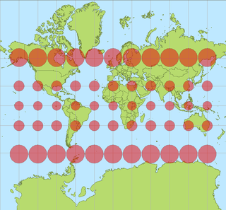
In cartography, a Tissot's indicatrix is a mathematical contrivance presented by French mathematician Nicolas Auguste Tissot in 1859 and 1871 in order to characterize local distortions due to map projection. It is the geometry that results from projecting a circle of infinitesimal radius from a curved geometric model, such as a globe, onto a map. Tissot proved that the resulting diagram is an ellipse whose axes indicate the two principal directions along which scale is maximal and minimal at that point on the map.

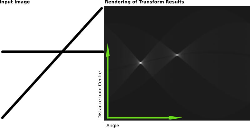
The generalized Hough transform (GHT), introduced by Dana H. Ballard in 1981, is the modification of the Hough transform using the principle of template matching. The Hough transform was initially developed to detect analytically defined shapes. In these cases, we have knowledge of the shape and aim to find out its location and orientation in the image. This modification enables the Hough transform to be used to detect an arbitrary object described with its model.

<span class="mw-page-title-main">Kepler orbit</span> Celestial orbit whose trajectory is a conic section in the orbital plane

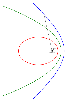
In celestial mechanics, a Kepler orbit is the motion of one body relative to another, as an ellipse, parabola, or hyperbola, which forms a two-dimensional orbital plane in three-dimensional space. A Kepler orbit can also form a straight line. It considers only the point-like gravitational attraction of two bodies, neglecting perturbations due to gravitational interactions with other objects, atmospheric drag, solar radiation pressure, a non-spherical central body, and so on. It is thus said to be a solution of a special case of the two-body problem, known as the Kepler problem. As a theory in classical mechanics, it also does not take into account the effects of general relativity. Keplerian orbits can be parametrized into six orbital elements in various ways.

Hough transforms are techniques for object detection, a critical step in many implementations of computer vision, or data mining from images. Specifically, the Randomized Hough transform is a probabilistic variant to the classical Hough transform, and is commonly used to detect curves The basic idea of Hough transform (HT) is to implement a voting procedure for all potential curves in the image, and at the termination of the algorithm, curves that do exist in the image will have relatively high voting scores. Randomized Hough transform (RHT) is different from HT in that it tries to avoid conducting the computationally expensive voting process for every nonzero pixel in the image by taking advantage of the geometric properties of analytical curves, and thus improve the time efficiency and reduce the storage requirement of the original algorithm.

Chessboards arise frequently in computer vision theory and practice because their highly structured geometry is well-suited for algorithmic detection and processing. The appearance of chessboards in computer vision can be divided into two main areas: camera calibration and feature extraction. This article provides a unified discussion of the role that chessboards play in the canonical methods from these two areas, including references to the seminal literature, examples, and pointers to software implementations.

The circle Hough Transform (CHT) is a basic feature extraction technique used in digital image processing for detecting circles in imperfect images. The circle candidates are produced by “voting” in the Hough parameter space and then selecting local maxima in an accumulator matrix.

In image analysis, the generalized structure tensor (GST) is an extension of the Cartesian structure tensor to curvilinear coordinates. It is mainly used to detect and to represent the "direction" parameters of curves, just as the Cartesian structure tensor detects and represents the direction in Cartesian coordinates. Curve families generated by pairs of locally orthogonal functions have been the best studied.

In image processing, line detection is an algorithm that takes a collection of n edge points and finds all the lines on which these edge points lie. The most popular line detectors are the Hough transform and convolution-based techniques.

References

  1. Shapiro, Linda and Stockman, George. "Computer Vision", Prentice-Hall, Inc. 2001
  2. Romanengo, Chiara; Falcidieno, Bianca; Biasotti, Silvia (2024-09-01). "Extending the Hough transform to recognize and approximate space curves in 3D models". Computer Aided Geometric Design. 113: 102377. doi:10.1016/j.cagd.2024.102377. ISSN   0167-8396.
  3. Duda, R. O. and P. E. Hart, "Use of the Hough Transformation to Detect Lines and Curves in Pictures," Comm. ACM, Vol. 15, pp. 11–15 (January, 1972)
  4. Hough, P.V.C. Method and means for recognizing complex patterns, U.S. Patent 3,069,654, Dec. 18, 1962
  5. P.V.C. Hough, Machine Analysis of Bubble Chamber Pictures, Proc. Int. Conf. High Energy Accelerators and Instrumentation, 1959
  6. Richard O. Duda; Peter E. Hart (April 1971). "Use of the Hough Transformation to Detect Lines and Curves in Pictures" (PDF). Artificial Intelligence Center .
  7. A short introduction to the Radon and Hough transforms and how they relate to each other. CiteSeerX.
  8. Stephens, R. S. (1990). "A probabilistic approach to the Hough Transform". Proceedings of the British Machine Vision Conference 1990. British Machine Vision Association: 12.1–12.6. doi:10.5244/c.4.12.
  9. Jensen, Jeppe. "Hough Transform for Straight Lines" (PDF). Archived from the original (PDF) on 26 April 2012. Retrieved 16 December 2011.
  10. Fernandes, L.A.F.; Oliveira, M.M. (2008). "Real-time line detection through an improved Hough transform voting scheme". Pattern Recognition. 41 (1): 299–314. Bibcode:2008PatRe..41..299F. doi:10.1016/j.patcog.2007.04.003. S2CID   5996185.
  11. Limberger, F. A.; Oliveira, M. M. (2015). "Real-Time Detection of Planar Regions in Unorganized Point Clouds" (PDF). Pattern Recognition. 48 (6): 2043–2053. Bibcode:2015PatRe..48.2043L. doi:10.1016/j.patcog.2014.12.020. hdl: 10183/97001 .
  12. Fernandes, L.A.F.; Oliveira, M.M. (2012). "A general framework for subspace detection in unordered multidimensional data". Pattern Recognition. 45 (9): 3566–3579. Bibcode:2012PatRe..45.3566F. doi:10.1016/j.patcog.2012.02.033.
  13. Ballard, D.H. (1981). "Generalizing the Hough transform to detect arbitrary shapes". Pattern Recognition. 13 (2): 111–122. Bibcode:1981PatRe..13..111B. doi:10.1016/0031-3203(81)90009-1. hdl: 1802/13802 .
  14. Vosselman, G., Dijkman, S: "3D Building Model Reconstruction from Point Clouds and Ground Plans", International Archives of the Photogrammetry, Remote Sensing and Spatial Information Sciences, vol 34, part 3/W4, October 22–24, 2001, Annapolis, MA, USA, pp. 37–44.
  15. Tahir Rabbani: "Automatic reconstruction of industrial installations – Using point clouds and images" Archived 2008-12-01 at the Wayback Machine , pages 43–44, Publications on Geodesy 62, Delft, 2006. ISBN   978-90-6132-297-9.
  16. Achtert, Elke; Böhm, Christian; David, Jörn; Kröger, Peer; Zimek, Arthur (2008). "Global Correlation Clustering Based on the Hough Transform". Statistical Analysis and Data Mining. 1 (3): 111–127. CiteSeerX   10.1.1.716.6006 . doi:10.1002/sam.10012. S2CID   5111283.
  17. Tahir Rabbani and Frank van den Heuvel, "Efficient hough transform for automatic detection of cylinders in point clouds" in Proceedings of the 11th Annual Conference of the Advanced School for Computing and Imaging (ASCI '05), The Netherlands, June 2005.
  18. Yonghong Xie; Qiang Ji (2002). "A new efficient ellipse detection method". Object recognition supported by user interaction for service robots. Vol. 2. pp. 957–960. CiteSeerX   10.1.1.1.8792 . doi:10.1109/ICPR.2002.1048464. ISBN   978-0-7695-1695-0. S2CID   9276255.
  19. "Image Transforms - Hough Transform". Homepages.inf.ed.ac.uk. Retrieved 2009-08-17.