A Fourier transform (FT) is a mathematical transform that decomposes functions depending on space or time into functions depending on spatial frequency or temporal frequency. That process is also called analysis. An example application would be decomposing the waveform of a musical chord into terms of the intensity of its constituent pitches. The term Fourier transform refers to both the frequency domain representation and the mathematical operation that associates the frequency domain representation to a function of space or time.
In the mathematical field of complex analysis, elliptic functions are a special kind of meromorphic functions, that satisfy two periodicity conditions. They are named elliptic functions because they come from elliptic integrals. Originally those integrals occurred at the calculation of the arc length of an ellipse.
In mathematics, a self-adjoint operator on an infinite-dimensional complex vector space V with inner product is a linear map A that is its own adjoint. If V is finite-dimensional with a given orthonormal basis, this is equivalent to the condition that the matrix of A is a Hermitian matrix, i.e., equal to its conjugate transpose A∗. By the finite-dimensional spectral theorem, V has an orthonormal basis such that the matrix of A relative to this basis is a diagonal matrix with entries in the real numbers. In this article, we consider generalizations of this concept to operators on Hilbert spaces of arbitrary dimension.
In the mathematical field of representation theory, a weight of an algebra A over a field F is an algebra homomorphism from A to F, or equivalently, a one-dimensional representation of A over F. It is the algebra analogue of a multiplicative character of a group. The importance of the concept, however, stems from its application to representations of Lie algebras and hence also to representations of algebraic and Lie groups. In this context, a weight of a representation is a generalization of the notion of an eigenvalue, and the corresponding eigenspace is called a weight space.

In physics, the reciprocal lattice represents the Fourier transform of another lattice. In normal usage, the initial lattice is usually a periodic spatial function in real-space and is also known as the direct lattice. While the direct lattice exists in real-space and is what one would commonly understand as a physical lattice, the reciprocal lattice exists in reciprocal space. The reciprocal lattice of a reciprocal lattice is equivalent to the original direct lattice, because the defining equations are symmetrical with respect to the vectors in real and reciprocal space. Mathematically, direct and reciprocal lattice vectors represent covariant and contravariant vectors, respectively.

In the physical sciences and electrical engineering, dispersion relations describe the effect of dispersion on the properties of waves in a medium. A dispersion relation relates the wavelength or wavenumber of a wave to its frequency. Given the dispersion relation, one can calculate the phase velocity and group velocity of waves in the medium, as a function of frequency. In addition to the geometry-dependent and material-dependent dispersion relations, the overarching Kramers–Kronig relations describe the frequency dependence of wave propagation and attenuation.
In functional analysis, a branch of mathematics, the Borel functional calculus is a functional calculus, which has particularly broad scope. Thus for instance if T is an operator, applying the squaring function s → s2 to T yields the operator T2. Using the functional calculus for larger classes of functions, we can for example define rigorously the "square root" of the (negative) Laplacian operator −Δ or the exponential
In physics and mathematics, supermanifolds are generalizations of the manifold concept based on ideas coming from supersymmetry. Several definitions are in use, some of which are described below.
In statistics and probability theory, a point process or point field is a collection of mathematical points randomly located on a mathematical space such as the real line or Euclidean space. Point processes can be used for spatial data analysis, which is of interest in such diverse disciplines as forestry, plant ecology, epidemiology, geography, seismology, materials science, astronomy, telecommunications, computational neuroscience, economics and others.
In mathematics, the Gibbs measure, named after Josiah Willard Gibbs, is a probability measure frequently seen in many problems of probability theory and statistical mechanics. It is a generalization of the canonical ensemble to infinite systems. The canonical ensemble gives the probability of the system X being in state x as

Wigner's theorem, proved by Eugene Wigner in 1931, is a cornerstone of the mathematical formulation of quantum mechanics. The theorem specifies how physical symmetries such as rotations, translations, and CPT are represented on the Hilbert space of states.
In mathematics, Lindelöf's theorem is a result in complex analysis named after the Finnish mathematician Ernst Leonard Lindelöf. It states that a holomorphic function on a half-strip in the complex plane that is bounded on the boundary of the strip and does not grow "too fast" in the unbounded direction of the strip must remain bounded on the whole strip. The result is useful in the study of the Riemann zeta function, and is a special case of the Phragmén–Lindelöf principle. Also, see Hadamard three-lines theorem.
Linear Programming Boosting (LPBoost) is a supervised classifier from the boosting family of classifiers. LPBoost maximizes a margin between training samples of different classes and hence also belongs to the class of margin-maximizing supervised classification algorithms. Consider a classification function
In mathematics, the spectral theory of ordinary differential equations is the part of spectral theory concerned with the determination of the spectrum and eigenfunction expansion associated with a linear ordinary differential equation. In his dissertation Hermann Weyl generalized the classical Sturm–Liouville theory on a finite closed interval to second order differential operators with singularities at the endpoints of the interval, possibly semi-infinite or infinite. Unlike the classical case, the spectrum may no longer consist of just a countable set of eigenvalues, but may also contain a continuous part. In this case the eigenfunction expansion involves an integral over the continuous part with respect to a spectral measure, given by the Titchmarsh–Kodaira formula. The theory was put in its final simplified form for singular differential equations of even degree by Kodaira and others, using von Neumann's spectral theorem. It has had important applications in quantum mechanics, operator theory and harmonic analysis on semisimple Lie groups.
In mathematics, the Schauder estimates are a collection of results due to Juliusz Schauder concerning the regularity of solutions to linear, uniformly elliptic partial differential equations. The estimates say that when the equation has appropriately smooth terms and appropriately smooth solutions, then the Hölder norm of the solution can be controlled in terms of the Hölder norms for the coefficient and source terms. Since these estimates assume by hypothesis the existence of a solution, they are called a priori estimates.

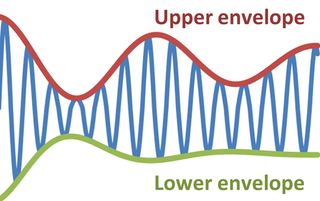
In physics and engineering, the envelope of an oscillating signal is a smooth curve outlining its extremes. The envelope thus generalizes the concept of a constant amplitude into an instantaneous amplitude. The figure illustrates a modulated sine wave varying between an upper envelope and a lower envelope. The envelope function may be a function of time, space, angle, or indeed of any variable.
In the mathematical fields of numerical analysis and approximation theory, box splines are piecewise polynomial functions of several variables. Box splines are considered as a multivariate generalization of basis splines (B-splines) and are generally used for multivariate approximation/interpolation. Geometrically, a box spline is the shadow (X-ray) of a hypercube projected down to a lower-dimensional space. Box splines and simplex splines are well studied special cases of polyhedral splines which are defined as shadows of general polytopes.
In probability theory, an interacting particle system (IPS) is a stochastic process on some configuration space given by a site space, a countable-infinite graph and a local state space, a compact metric space . More precisely IPS are continuous-time Markov jump processes describing the collective behavior of stochastically interacting components. IPS are the continuous-time analogue of stochastic cellular automata.
A multidimensional signal is a function of M independent variables where . Real world signals, which are generally continuous time signals, have to be discretized (sampled) in order to ensure that digital systems can be used to process the signals. It is during this process of discretization where sampling comes into picture. Although there are many ways of obtaining a discrete representation of a continuous time signal, periodic sampling is by far the simplest scheme. Theoretically, sampling can be performed with respect to any set of points. But practically, sampling is carried out with respect to a set of points that have a certain algebraic structure. Such structures are called lattices. Mathematically, the process of sampling an -dimensional signal can be written as:
The quaternion estimator algorithm (QUEST) is an algorithm designed to solve Wahba's problem, that consists of finding a rotation matrix between two coordinate systems from two sets of observations sampled in each system respectively. The key idea behind the algorithm is to find an expression of the loss function for the Wahba's problem as a quadratic form, using the Cayley–Hamilton theorem and the Newton–Raphson method to efficiently solve the eigenvalue problem and construct a numerically stable representation of the solution.


![Fig. 3: Support of the sampled spectrum
f
^
s
(
[?]
)
{\displaystyle {\hat {f}}_{s}(\cdot )}
obtained by hexagonal sampling of a two-dimensional function wavenumber-limited to a circular disc. The blue circle represents the support
O
{\displaystyle \Omega }
of the original wavenumber-limited field, and the green circles represent the repetitions. In this example the spectral repetitions do not overlap and hence there is no aliasing. The original spectrum can be exactly recovered from the sampled spectrum. Unaliased sampled spectrum in 2D.png](http://upload.wikimedia.org/wikipedia/en/thumb/4/42/Unaliased_sampled_spectrum_in_2D.png/300px-Unaliased_sampled_spectrum_in_2D.png)


![Fig. 4: Support of the sampled spectrum
f
^
s
(
[?]
)
{\displaystyle {\hat {f}}_{s}(\cdot )}
obtained by hexagonal sampling of a two-dimensional function wavenumber-limited to a circular disc. In this example, the sampling lattice is not fine enough and hence the discs overlap in the sampled spectrum. Thus the spectrum within
O
{\displaystyle \Omega }
represented by the blue circle cannot be recovered exactly due to the overlap from the repetitions (shown in green), thus leading to aliasing. Aliased sampled spectrum in 2D.png](http://upload.wikimedia.org/wikipedia/commons/thumb/d/df/Aliased_sampled_spectrum_in_2D.png/300px-Aliased_sampled_spectrum_in_2D.png)


