Primary line constants

Last updated

Telephone cable containing multiple twisted-pair lines Telephone cable.jpg
Telephone cable containing multiple twisted-pair lines

The primary line constants are parameters that describe the characteristics of conductive transmission lines, such as pairs of copper wires, in terms of the physical electrical properties of the line. The primary line constants are only relevant to transmission lines and are to be contrasted with the secondary line constants, which can be derived from them, and are more generally applicable. The secondary line constants can be used, for instance, to compare the characteristics of a waveguide to a copper line, whereas the primary constants have no meaning for a waveguide.

Contents

The constants are conductor resistance and inductance, and insulator capacitance and conductance, which are by convention given the symbols R, L, C, and G respectively. The constants are enumerated in terms of per unit length. The circuit representation of these elements requires a distributed-element model and consequently calculus must be used to analyse the circuit. The analysis yields a system of two first order, simultaneous linear partial differential equations which may be combined to derive the secondary constants of characteristic impedance and propagation constant.

A number of special cases have particularly simple solutions and important practical applications. Low loss cable requires only L and C to be included in the analysis, useful for short lengths of cable. Low frequency applications, such as twisted pair telephone lines, are dominated by R and C only. High frequency applications, such as RF co-axial cable, are dominated by L and C. Lines loaded to prevent distortion need all four elements in the analysis, but have a simple, elegant solution.

The constants

There are four primary line constants, but in some circumstances some of them are small enough to be ignored and the analysis can be simplified. These four, and their symbols and units are as follows:

NameSymbolUnitsUnit symbol
loop resistance R ohms per metre Ω/m
loop inductance L henries per metreH/m
insulator capacitance C farads per metreF/m
insulator conductance G siemens per metreS/m

R and L are elements in series with the line (because they are properties of the conductor) and C and G are elements shunting the line (because they are properties of the dielectric material between the conductors). G represents leakage current through the dielectric and in most cables is very small. The word loop is used to emphasise that the resistance and inductance of both conductors must be taken into account. For instance, if a line consists of two identical wires that have a resistance of 25 mΩ/m each, the loop resistance is double that, 50 mΩ/m. Because the values of the constants are quite small, it is common for manufacturers to quote them per kilometre rather than per metre; in the English-speaking world "per mile" can also be used. [1] [2]

The word "constant" can be misleading. It means that they are material constants; but they may vary with frequency. In particular, R is heavily influenced by the skin effect. Furthermore, while G has virtually no effect at audio frequency, it can cause noticeable losses at high frequency with many of the dielectric materials used in cables due to a high loss tangent. Avoiding the losses caused by G is the reason many cables designed for use at UHF are air-insulated or foam-insulated (which makes them virtually air-insulated). [3] The actual meaning of constant in this context is that the parameter is constant with distance. That is the line is assumed to be homogenous lengthwise. This condition is true for the vast majority of transmission lines in use today. [4]

Typical values for some common cables

DesignationCable formApplicationRLGCZ0
Ω/kmμH/kmnS/kmnF/kmΩ
CAT5 [5] Twisted pair Data transmission 176490<249100
CAT5e [6] Twisted pairData transmission176<2100
CW1308 [7] Twisted pair Telephony 98<20
RG59 [8] Coaxial Video364306975
RG59 [9] Coaxial
(foam dielectric)
Video 173035475
RG58 [10] [11] Coaxial Radio frequency 48253<0.0110150
Low loss [12] Coaxial
(Foam dielectric)
Radio frequency
transmitter feed
2.861887550
DIN VDE 0816 [13] Star quadTelephony
(trunk lines)
31.8<0.135
† Manufacturers commonly omit a value for inductance in their data sheets. Some of these values are estimated from the figures for capacitance and characteristic impedance by .

Circuit representation

Fig. 1. Equivalent circuit representation of a transmission line using distributed elements. dL, dR, dC and dG are to be read as, Ldx, Rdx, Cdx and Gdx respectively Line model Heaviside.svg
Fig. 1. Equivalent circuit representation of a transmission line using distributed elements. δL, δR, δC and δG are to be read as, Lδx, Rδx, Cδx and Gδx respectively

The line constants cannot be simply represented as lumped elements in a circuit; they must be described as distributed elements. For instance "pieces" of the capacitance are in between "pieces" of the resistance. However many pieces the R and C are broken into, it can always be argued they should be broken apart further to properly represent the circuit, and after each division the number of meshes in the circuit is increased. This is shown diagramtically in figure 1. To give a true representation of the circuit, the elements must be made infinitesimally small so that each element is distributed along the line. The infinitesimal elements in an infinitesimal distance are given by; [14]


Fig. 2. Representation of a transmission line using generalised distributed impedance and admittance elements. Line model general impedances.svg
Fig. 2. Representation of a transmission line using generalised distributed impedance and admittance elements.

It is convenient for the purposes of analysis to roll up these elements into general series impedance, Z, and shunt admittance, Y elements such that;

and,

Analysis of this network (figure 2) will yield the secondary line constants: the propagation constant, , (whose real and imaginary parts are the attenuation constant, , and phase change constant, , respectively) and the characteristic impedance, , which also, in general, will have real, , and imaginary, , parts, making a total of four secondary constants to be derived from the four primary constants. The term constant is even more misleading for the secondary constants as they usually vary quite strongly with frequency, even in an ideal situation where the primary constants do not. This is because the reactances in the circuit ( and ) introduce a dependence on . It is possible to choose specific values of the primary constants that result in and being independent of (the Heaviside condition) but even in this case, there is still which is directly proportional to . As with the primary constants, the meaning of "constant" is that the secondary constants do not vary with distance along the line, not that they are independent of frequency. [14] [15] [16]

Characteristic impedance

Fig. 3. Equivalent circuit of a transmission line for the calculation of Z0 from the primary line constants Line equivalent circuit for Zo.svg
Fig. 3. Equivalent circuit of a transmission line for the calculation of Z0 from the primary line constants

The characteristic impedance of a transmission line, , is defined as the impedance looking into an infinitely long line. Such a line will never return a reflection since the incident wave will never reach the end to be reflected. When considering a finite length of the line, the remainder of the line can be replaced by as its equivalent circuit. This is so because the remainder of the line is still infinitely long and therefore equivalent to the original line. If the finite segment is very short, then in the equivalent circuit it will be modelled by an L-network consisting of one element of and one of ; the remainder is given by . This results in the network shown in figure 3, which can be analysed for using the usual network analysis theorems, [17] [18]

which re-arranges to,

Taking limits of both sides

and since the line was assumed to be homogenous lengthwise,

Propagation constant

Fig. 4. Each infinitesimal section of the transmission line causes an infinitesimal drop in the line voltage as it is propagated along the line. Integrating these drops enables the propagation constant to be found. Calculation of transmission line propagation constant.svg
Fig. 4. Each infinitesimal section of the transmission line causes an infinitesimal drop in the line voltage as it is propagated along the line. Integrating these drops enables the propagation constant to be found.

The ratio of the line input voltage to the voltage a distance further down the line (that is, after one section of the equivalent circuit) is given by a standard voltage divider calculation. The remainder of the line to the right, as in the characteristic impedance calculation, is replaced with , [19] [20]

Each infinitesimal section will multiply the voltage drop by the same factor. After sections the voltage ratio will be,

At a distance along the line, the number of sections is so that,

In the limit as ,

The second order term will disappear in the limit, so we can write without loss of accuracy,

and comparing with the mathematical identity,

yields,

From the definition of propagation constant,

Hence,

Special cases

Ideal transmission line

An ideal transmission line will have no loss, which implies that the resistive elements are zero. It also results in a purely real (resistive) characteristic impedance. The ideal line cannot be realised in practice, but it is a useful approximation in many circumstances. This is especially true, for instance, when short pieces of line are being used as circuit components such as stubs. A short line has very little loss and this can then be ignored and treated as an ideal line. The secondary constants in these circumstances are; [21]

Twisted pair

Typically, twisted pair cable used for audio frequencies or low data rates has line constants dominated by R and C. The dielectric loss is usually negligible at these frequencies and G is close to zero. It is also the case that, at a low enough frequency, which means that L can also be ignored. In those circumstances the secondary constants become, [22]

The attenuation of this cable type increases with frequency, causing distortion of waveforms. Not so obviously, the variation of with frequency also causes a distortion of a type called dispersion. To avoid dispersion the requirement is that is directly proportional to . However, it is actually proportional to and dispersion results. also varies with frequency and is also partly reactive; both these features will be the cause of reflections from a resistive line termination. This is another undesirable effect. The nominal impedance quoted for this type of cable is, in this case, very nominal, being valid at only one spot frequency, usually quoted at 800 Hz or 1 kHz. [23] [24]

Co-axial cable

Cable operated at a high enough frequency (medium wave radio frequency or high data rates) will meet the conditions and . This must eventually be the case as the frequency is increased for any cable. Under those conditions R and G can both be ignored (except for the purpose of calculating the cable loss) and the secondary constants become; [25]

Loaded line

Loaded lines are lines designed with deliberately increased inductance. This is done by adding iron or some other magnetic metal to the cable or adding coils. The purpose is to ensure that the line meets the Heaviside condition, which eliminates distortion caused by frequency-dependent attenuation and dispersion, and ensures that is constant and resistive. The secondary constants are here related to the primary constants by; [26]

Velocity

The velocity of propagation is given by,

Since,

and

then,

In cases where β can be taken as,

the velocity of propagation is given by,

The lower the capacitance the higher the velocity. With an air dielectric cable, which is approximated to with low-loss cable, the velocity of propagation is very close to c, the speed of light in vacuo. [27]

Notes

  1. Connor, p. 8.
  2. Bird, pp. 604–605.
  3. Porges, pp. 223–224.
  4. Bird, pp. 502–503, 519.
  5. "Bulk cable - Category 5 UTP 4-pair PVC", Molex data sheet, 1999, archived 7 August 2013.
  6. "1583E CAT5E UTP PVC", Belden data sheet 46077, 21 July 1999, archived 7 August 2013.
  7. "CW1308 Internal Telecom Cable" Archived 4 March 2016 at the Wayback Machine , Eland Cables data sheets, archived 8 August 2013.
  8. "8281 Coax - Double Braided RG-59/U Type" Belden data sheet, 14 May 2007, archived 7 August 2013.
  9. "Serial digital video cable", Belden data sheet 1865A, archived 7 August 2013.
  10. "Suhner coaxial cable", Huber & Suhner data sheet, 24 September 2007, archived 7 August 2013.
  11. "RG58/U" Archived 7 October 2009 at the Wayback Machine , General Cable datasheet, pp. 74–76.
  12. "7/8" Cellflex Lite Low-Loss Foam-Dielectric Coaxial Cable", RFS datasheet LCF78-50JFNL, 24 October 2006, archived 7 August 2013.
  13. "Trunk cables, paper insulated with aluminium sheath" Archived 30 November 2013 at the Wayback Machine , Nexus datasheet, archived 7 August 2013.
  14. 1 2 Connor, pp. 8–10.
  15. Hickman, p. 113.
  16. Porges, p. 217.
  17. Porges, pp. 216–217.
  18. Connor, pp. 10–11.
  19. Connor, pp. 9–10.
  20. Bird, pp. 609–611.
  21. Connor, p. 17.
  22. Connor, pp. 18–19.
  23. Bird, pp. 612–613.
  24. Porges, p. 219.
  25. Connor, p. 19.
  26. Connor, pp. 19–21.
  27. Connor, pp. 10, 19-20.

Related Research Articles

<span class="mw-page-title-main">Oscillation</span> Repetitive variation of some measure about a central value

Oscillation is the repetitive or periodic variation, typically in time, of some measure about a central value or between two or more different states. Familiar examples of oscillation include a swinging pendulum and alternating current. Oscillations can be used in physics to approximate complex interactions, such as those between atoms.

<span class="mw-page-title-main">Characteristic impedance</span> Property of an electrical circuit

The characteristic impedance or surge impedance (usually written Z0) of a uniform transmission line is the ratio of the amplitudes of voltage and current of a single wave propagating along the line; that is, a wave travelling in one direction in the absence of reflections in the other direction. Alternatively, and equivalently, it can be defined as the input impedance of a transmission line when its length is infinite. Characteristic impedance is determined by the geometry and materials of the transmission line and, for a uniform line, is not dependent on its length. The SI unit of characteristic impedance is the ohm.

The propagation constant of a sinusoidal electromagnetic wave is a measure of the change undergone by the amplitude and phase of the wave as it propagates in a given direction. The quantity being measured can be the voltage, the current in a circuit, or a field vector such as electric field strength or flux density. The propagation constant itself measures the dimensionless change in magnitude or phase per unit length. In the context of two-port networks and their cascades, propagation constant measures the change undergone by the source quantity as it propagates from one port to the next.

<span class="mw-page-title-main">Transmission line</span> Cable or other structure for carrying radio waves

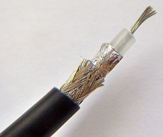
In electrical engineering, a transmission line is a specialized cable or other structure designed to conduct electromagnetic waves in a contained manner. The term applies when the conductors are long enough that the wave nature of the transmission must be taken into account. This applies especially to radio-frequency engineering because the short wavelengths mean that wave phenomena arise over very short distances. However, the theory of transmission lines was historically developed to explain phenomena on very long telegraph lines, especially submarine telegraph cables.

<span class="mw-page-title-main">Bremsstrahlung</span> Electromagnetic radiation due to deceleration of charged particles

In particle physics, bremsstrahlung is electromagnetic radiation produced by the deceleration of a charged particle when deflected by another charged particle, typically an electron by an atomic nucleus. The moving particle loses kinetic energy, which is converted into radiation, thus satisfying the law of conservation of energy. The term is also used to refer to the process of producing the radiation. Bremsstrahlung has a continuous spectrum, which becomes more intense and whose peak intensity shifts toward higher frequencies as the change of the energy of the decelerated particles increases.

In mathematics, the Hodge star operator or Hodge star is a linear map defined on the exterior algebra of a finite-dimensional oriented vector space endowed with a nondegenerate symmetric bilinear form. Applying the operator to an element of the algebra produces the Hodge dual of the element. This map was introduced by W. V. D. Hodge.

<span class="mw-page-title-main">Proper time</span> Elapsed time between two events as measured by a clock that passes through both events

In relativity, proper time along a timelike world line is defined as the time as measured by a clock following that line. The proper time interval between two events on a world line is the change in proper time, which is independent of coordinates, and is a Lorentz scalar. The interval is the quantity of interest, since proper time itself is fixed only up to an arbitrary additive constant, namely the setting of the clock at some event along the world line.

Acoustic impedance and specific acoustic impedance are measures of the opposition that a system presents to the acoustic flow resulting from an acoustic pressure applied to the system. The SI unit of acoustic impedance is the pascal-second per cubic metre, or in the MKS system the rayl per square metre, while that of specific acoustic impedance is the pascal-second per metre, or in the MKS system the rayl. There is a close analogy with electrical impedance, which measures the opposition that a system presents to the electric current resulting from a voltage applied to the system.

In mathematics, the discrete-time Fourier transform (DTFT) is a form of Fourier analysis that is applicable to a sequence of discrete values.

A transmission line which meets the Heaviside condition, named for Oliver Heaviside (1850–1925), and certain other conditions can transmit signals without dispersion and without distortion. The importance of the Heaviside condition is that it showed the possibility of dispersionless transmission of telegraph signals.In some cases, the performance of a transmission line can be improved by adding inductive loading to the cable.

In calculus, the Leibniz integral rule for differentiation under the integral sign states that for an integral of the form

<span class="mw-page-title-main">Stub (electronics)</span> Short electrical transmission line

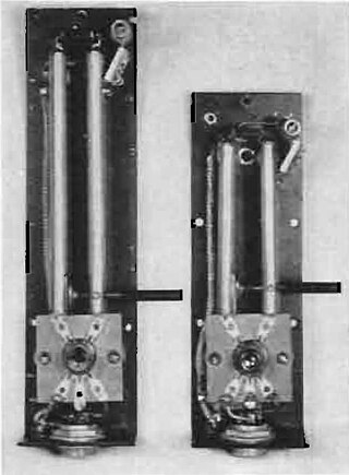
In microwave and radio-frequency engineering, a stub or resonant stub is a length of transmission line or waveguide that is connected at one end only. The free end of the stub is either left open-circuit, or short-circuited. Neglecting transmission line losses, the input impedance of the stub is purely reactive; either capacitive or inductive, depending on the electrical length of the stub, and on whether it is open or short circuit. Stubs may thus function as capacitors, inductors and resonant circuits at radio frequencies.

<span class="mw-page-title-main">Duffing equation</span> Non-linear second order differential equation and its attractor

The Duffing equation, named after Georg Duffing (1861–1944), is a non-linear second-order differential equation used to model certain damped and driven oscillators. The equation is given by

The telegrapher's equations are a set of two coupled, linear equations that predict the voltage and current distributions on a linear electrical transmission line. The equations are important because they allow transmission lines to be analyzed using circuit theory. The equations and their solutions are applicable from 0 Hz to frequencies at which the transmission line structure can support higher order non-TEM modes. The equations can be expressed in both the time domain and the frequency domain. In the time domain the independent variables are distance and time. The resulting time domain equations are partial differential equations of both time and distance. In the frequency domain the independent variables are distance and either frequency, or complex frequency, The frequency domain variables can be taken as the Laplace transform or Fourier transform of the time domain variables or they can be taken to be phasors. The resulting frequency domain equations are ordinary differential equations of distance. An advantage of the frequency domain approach is that differential operators in the time domain become algebraic operations in frequency domain.

In optics, the term soliton is used to refer to any optical field that does not change during propagation because of a delicate balance between nonlinear and dispersive effects in the medium. There are two main kinds of solitons:

<span class="mw-page-title-main">Zobel network</span>

Zobel networks are a type of filter section based on the image-impedance design principle. They are named after Otto Zobel of Bell Labs, who published a much-referenced paper on image filters in 1923. The distinguishing feature of Zobel networks is that the input impedance is fixed in the design independently of the transfer function. This characteristic is achieved at the expense of a much higher component count compared to other types of filter sections. The impedance would normally be specified to be constant and purely resistive. For this reason, Zobel networks are also known as constant resistance networks. However, any impedance achievable with discrete components is possible.

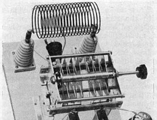
Constant k filters, also k-type filters, are a type of electronic filter designed using the image method. They are the original and simplest filters produced by this methodology and consist of a ladder network of identical sections of passive components. Historically, they are the first filters that could approach the ideal filter frequency response to within any prescribed limit with the addition of a sufficient number of sections. However, they are rarely considered for a modern design, the principles behind them having been superseded by other methodologies which are more accurate in their prediction of filter response.

m-derived filters or m-type filters are a type of electronic filter designed using the image method. They were invented by Otto Zobel in the early 1920s. This filter type was originally intended for use with telephone multiplexing and was an improvement on the existing constant k type filter. The main problem being addressed was the need to achieve a better match of the filter into the terminating impedances. In general, all filters designed by the image method fail to give an exact match, but the m-type filter is a big improvement with suitable choice of the parameter m. The m-type filter section has a further advantage in that there is a rapid transition from the cut-off frequency of the passband to a pole of attenuation just inside the stopband. Despite these advantages, there is a drawback with m-type filters; at frequencies past the pole of attenuation, the response starts to rise again, and m-types have poor stopband rejection. For this reason, filters designed using m-type sections are often designed as composite filters with a mixture of k-type and m-type sections and different values of m at different points to get the optimum performance from both types.

<span class="mw-page-title-main">RLC circuit</span> Resistor Inductor Capacitor Circuit

An RLC circuit is an electrical circuit consisting of a resistor (R), an inductor (L), and a capacitor (C), connected in series or in parallel. The name of the circuit is derived from the letters that are used to denote the constituent components of this circuit, where the sequence of the components may vary from RLC.

<span class="mw-page-title-main">Loop-gap resonator</span>

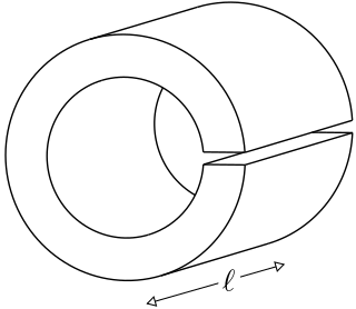
A loop-gap resonator (LGR) is an electromagnetic resonator that operates in the radio and microwave frequency ranges. The simplest LGRs are made from a conducting tube with a narrow slit cut along its length. The LGR dimensions are typically much smaller than the free-space wavelength of the electromagnetic fields at the resonant frequency. Therefore, relatively compact LGRs can be designed to operate at frequencies that are too low to be accessed using, for example, cavity resonators. These structures can have very sharp resonances making them useful for electron spin resonance (ESR) experiments, and precision measurements of electromagnetic material properties.

References